From a cpo to the category \mathbf {Cpo} [dt-004O]
Problem.
The following definitions are insufficient when using function constructions in our domain equations (\twoheadrightarrow and \mathbin {\circ \hspace{-0.4em}\twoheadrightarrow }), but it will suffice for our purposes for now.
Let us say (for now) that a cpo A approximates a cpo B (i.e. A \sqsubseteq B) iff there is a continuous function f : A\twoheadrightarrow B. Then, there is a least element for this ordering: the one-element cpo \mathbf {1} = \{ \bot \}, as the continuous function (\lambda x. \bot ) : \mathbf {1} \twoheadrightarrow A exists for any cpo A.
Categorical Aside. Initiality
The category \mathbf {Cpo} has no initial object. The cpo \mathbf {1} is terminal; but also serves as a "pseudo" initial object due to the above.
Colimits in the category \mathbf {Cpo} [dt-004P]
Definition\omega -chains of cpos in the category \mathbf {Cpo} [dt-004Q]
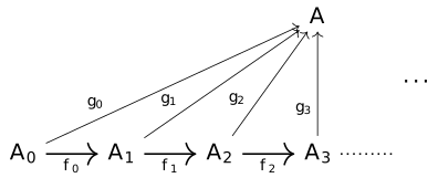
An \omega -chain of cpos in the category \mathbf {Cpo} consists of a family of cpos \{A_i \mid i \in \mathbb {N} \}, together with a family of continuous functions \{ f_i : A_i\twoheadrightarrow A_{i+1} \mid i \in \mathbb {N}\}, shown below:

DefinitionUpper bounds in the category \mathbf {Cpo} [dt-004R]
A cpo A is an upper bound of an \omega -chain of cpos in the category \mathbf {Cpo} if there is a family of continuous functions \{g_i : A_i \twoheadrightarrow A \mid i \in \mathbb {N}\} such that the following diagram commutes (i.e. g_i = g_{i+1} \circ f_i for all i \in \mathbb {N}):
DefinitionLeast upper bounds in the category \mathbf {Cpo} [dt-004S]
A cpo A is the least upper bound of an \omega -chain of cpos if is both an upper bound and if there exists a unique k for any other upper bound B such that the following diagram commutes (i.e. h_i = k \circ g_i for all i \in \mathbb {N}):
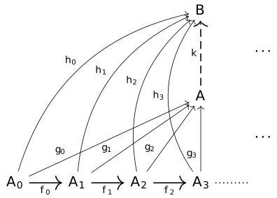
The least upper bound of such an \omega -chain is also called its colimit.
Note: Uniqueness of lubs is up to isomorphism. That is, if A and B are both colimits of our \omega -chain, then A \simeq B.
DefinitionEndofunctors on \textbf {Cpo} [dt-004T]
An endofunctor on the category \textbf {Cpo} is a functor \textbf {Cpo} \rightarrow \textbf {Cpo}, i.e. a mapping \mathcal {F} on cpos together with a mapping \mathcal {F} on continuous functions, such that:
- If f : A \twoheadrightarrow B then \mathcal {F}(f) : \mathcal {F}(A)\twoheadrightarrow \mathcal {F}(B)
- \mathcal {F}(\mathsf {id}_A : A\twoheadrightarrow A) = \mathsf {id}_{\mathcal {F}(A)} : \mathcal {F}(A)\twoheadrightarrow \mathcal {F}(A)
- \mathcal {F}(f \circ g) = \mathcal {F}(f) \circ \mathcal {F}(g)
Remark [dt-004U]
Observe that, given the information ordering for cpos where A \sqsubseteq B if there exists a continuous function A \twoheadrightarrow B, the functor laws necessarily imply monotonicity for all endofunctors \mathcal {F}.
DefinitionCocontinuous endofunctors [dt-004V]
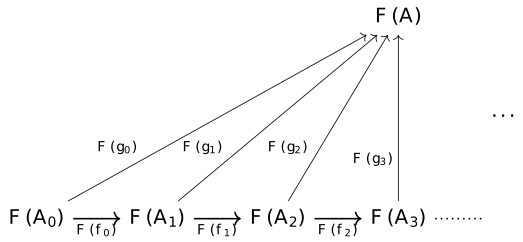
An endofunctor \mathcal {F} is cocontinuous iff it preserves colimits of \omega -chains of cpos. That is, given a chain where A is a colimit:
DefinitionFixed points of endofunctors on \mathbf {Cpo} [dt-004W]
A fixed point of an endofunctor on cpos \mathcal {F} is a cpo \mathcal {F} such that \mathcal {F}(A) \simeq A.
Note.
In Scott's approach, which we follow here, our fixed points are up to isomorphism (suitable for languages with isorecursive types), but there are other approaches where they are equalities (suitable for languages with equirecursive types).
TheoremFixed point theorem for endofunctors on \mathbf {Cpo} [dt-004X]
Every cocontinuous endofunctor \mathcal {F} on cpos has a least fixed point, given by the colimit of the \omega -chain:

ExampleBinary Numbers [dt-004Y]
Consider the Haskell-style data type: \textbf {data}\ \mathit {Bin} = \mathsf {Zero}\ \mathit {Bin} \mid \mathsf {Empty} \mid \mathsf {One}\ \mathit {Bin} So, e.g. \mathsf {One}\ (\mathsf {Zero}\ (\mathsf {One}\ \mathsf {Empty})) : \mathit {Bin}.
The recursive domain equation is, expressed as a fixed point: B \simeq \mathcal {F}(B)\quad \text {where}\ \mathcal {F}(X) = X + \mathbf {1} + X We wish to show that \mathcal {F} is a cocontinuous endofunctor.
We have a mapping \mathcal {F} on cpos (objects of the category \textbf {Cpo}), but for it to be a functor we additionally need a mapping \mathcal {F} on continuous functions (morphisms of the category \textbf {Cpo}).
Recalling our sum construction, we may remember that sums are already a bifunctor \textbf {Cpo} \times \textbf {Cpo} \rightarrow \textbf {Cpo} (Theorem [dt-0038]). Thus, our mapping on continuous functions \mathcal {F} can be derived from our mapping on cpos \mathcal {F} by using the morphism mapping from the sum construction (Definition [dt-0037]). Given a continuous function f : A \twoheadrightarrow B, our morphism mapping is:
\begin {array}{l} \mathcal {F}(f) : \mathcal {F}(A)\twoheadrightarrow \mathcal {F}(B)\\ \mathcal {F}(f) \triangleq f + \mathsf {id}_\textbf {1} + f \end {array}Proof that this endofunctor is cocontinuous is left for the reader. Hence the semantics of the type \mathit {Bin}, i.e. \llbracket \mathit {Bin} \rrbracket : \textbf {Cpo} is the least fixed point of \mathcal {F}, i.e. the colimit of the \omega -chain:

Let us visualise this chain. Here the sum injections have been written as \textsf {Z, E, O} rather than (combinations of) \textsf {inl} and \textsf {inr} to keep the connection with the Haskell data type clear.
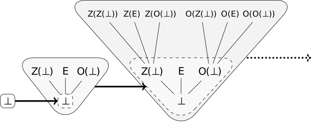
Thus, the nth cpo in the chain contains binary numbers with at most n defined digits. The colimit of the chain contains all binary numbers (finite, partial, and infinite!).
Exercise [dt-005M]
Show that \mathcal {F}(X) \triangleq \mathbf {1} + X and \mathcal {F}(f) \triangleq \mathsf {id}_\mathbf {1} + f (using our + operator for functions) define an endofunctor \mathbf {Cpo} \rightarrow \mathbf {Cpo}, i.e. that they satisfy the functor laws.
Solution.
- We must show \mathcal {F}(\mathsf {id}_A : A \twoheadrightarrow A) = \mathsf {id}_{\mathcal {F}(A)} : \mathcal {F}(A) \twoheadrightarrow \mathcal {F}(A). \begin {array}{lcl} \mathcal {F}(\mathsf {id}_A)& =& \mathsf {id}_\mathbf {1} + \mathsf {id}_A\\ &=& \mathsf {id}_{\mathbf {1} + A}\\ &=& \mathsf {id}_{\mathcal {F}(A)} \end {array}
- We must show \mathcal {F}(f \circ g) = \mathcal {F}(f) \circ \mathcal {F}(g). \begin {array}{lcl} \mathcal {F}(f \circ g) &=& \mathsf {id}_\mathbf {1} + (f \circ g) \\ &=& (\mathsf {id}_\mathbf {1} + f) \circ (\mathsf {id}_\mathbf {1} + g) \\ & = & \mathcal {F}(f) \circ \mathcal {F}(g) \end {array}
Constructing endofunctors [dt-0050]
If we have a mapping on cpos \mathcal {F} : \textbf {Cpo} \rightarrow \textbf {Cpo} that is made up of the primitives \times , +, \otimes , \oplus , \mathbf {1} and (\cdot )_\bot , we can generate a corresponding morphism mapping on continuous functions \mathcal {F} : (A\twoheadrightarrow B) \rightarrow (\mathcal {F}(A)\twoheadrightarrow \mathcal {F}(B)) by using the corresponding morphism mappings of each of these operators. Thus any such mapping can be turned into an endofunctor.
ExampleMaking endofunctors for algebraic data types [dt-0051]
\begin {array}{llr} \textsf {Object mapping} & \textsf {Morphism mapping}\\[0.2em] \mathcal {F}(X) = X + \mathbf {1} & \mathcal {F}(f) = f + \mathsf {id}_\mathbf {1} & \quad \quad \text {((co)-natural numbers)} \\ \mathcal {F}(X) = \mathbf {1} + (\mathbb {Z}_\bot \times X) & \mathcal {F}(f) = \mathsf {id}_\mathbf {1} + (\mathsf {id}_{\mathbb {Z}_\bot } \times f) & \text {((co)-lists of integers)}\\ \end {array}
Exercise [dt-005N]
The lazy natural numbers, also called conats, are defined as the least solution to the equation X \simeq \mathbf {1} + X.
- Sketch the first four approximations to the least fixed point. Call the two sum injections \mathsf {zero} and \mathsf {succ}.
Solution.
\begin {array}{lcl} A_0 & = & \{\bot \} \\ A_1 & = & \{\mathsf {zero}\ \bot , \mathsf {succ}\ \bot , \bot \} \\ A_2 & = & \{\mathsf {zero}\ \bot , \mathsf {succ}\ \bot , \mathsf {succ}\ (\mathsf {zero}\ \bot ), \mathsf {succ}\ (\mathsf {succ}\ \bot ), \bot \} \\ A_3 & = & \{\mathsf {zero}\ \bot , \mathsf {succ}\ \bot , \mathsf {succ}\ (\mathsf {zero}\ \bot ), \mathsf {succ}\ (\mathsf {succ}\ \bot ), \mathsf {succ}\ (\mathsf {succ}\ (\mathsf {zero}\ \bot )), \mathsf {succ}\ (\mathsf {succ}\ (\mathsf {succ}\ \bot )), \bot \} \\ \end {array} - Repeat this exercise assuming:
- \mathsf {zero} is strict (i.e. \mathsf {zero}\ \bot = \bot )
Solution.
\begin {array}{lcl} A_0 & = & \{\bot \} \\ A_1 & = & \{\mathsf {succ}\ \bot , \bot \} \\ A_2 & = & \{\mathsf {succ}\ \bot , \mathsf {succ}\ (\mathsf {succ}\ \bot ), \bot \} \\ A_3 & = & \{\mathsf {succ}\ \bot , \mathsf {succ}\ (\mathsf {succ}\ \bot ), \mathsf {succ}\ (\mathsf {succ}\ (\mathsf {succ}\ \bot )), \bot \} \\ \end {array} - \mathsf {succ} is strict (i.e. \mathsf {succ}\ \bot = \bot )
Solution.
\begin {array}{lcl} A_0 & = & \{\bot \} \\ A_1 & = & \{\mathsf {zero}\ \bot , \bot \} \\ A_2 & = & \{\mathsf {zero}\ \bot , \mathsf {succ}\ (\mathsf {zero}\ \bot ), \bot \} \\ A_3 & = & \{\mathsf {zero}\ \bot , \mathsf {succ}\ (\mathsf {zero}\ \bot ), \mathsf {succ}\ (\mathsf {succ}\ (\mathsf {zero}\ \bot )), \bot \} \\ \end {array}
- \mathsf {zero} is strict (i.e. \mathsf {zero}\ \bot = \bot )