Lecture. Domain theory › Recursively defined domains and \lambda -calculus [dt-004Z]
This lecture is based on material from Graham Hutton, John Longley, Dana Scott, Joseph Stoy, Carl Gunter, and Glynn Winskel.
Why we need recursively defined domains [dt-004J]
We saw recursive domain equations with higher-order procedures in § [dt-0007], but there are numerous other examples where they come up.
Recursive algebraic data types [dt-004L]
Suppose we have a language with recursive data types, such as this \mathit {List} type in Haskell-style syntax: \textbf {data}\ \mathit {List} = \mathsf {Nil} \mid \mathsf {Cons}\ (\mathit {Int} \times \mathit {List}) As in PCF, the denotation of a type \tau is the domain which contains all the denotations of all closed expressions of type \tau . What, then, is the domain that corresponds to \mathit {List}\ a? We need a cpo L that satisfies the below equation (where \mathbf {1} is the cpo containing just one element \bot ): L \simeq \mathbf {1} + (\mathbb {Z}_\bot \times L)
Untyped higher-order languages [dt-004M]
If we take PCF, discard the type system, \textbf {fix}, natural number primitives and any other superfluous features, and just boil our language down to a minimal, Turing-complete subset, we end up with the untyped \lambda -calculus — a language consisting only of untyped functions.
DefinitionUntyped \lambda -calculus [dt-004K]
Untyped \lambda -calculus consists only of untyped (higher-order) functions: e \; \Coloneqq \; x \mid \lambda x. e \mid e_1\ e_2
Trying to give a semantics to the untyped \lambda calculus poses an issue: we can no longer rely on the type of an expression to select an appropriate semantic domain. Instead, we we must pick a single domain D which, since functions can be applied to themselves, must apparently include the set of functions D \twoheadrightarrow D: D \simeq D\twoheadrightarrow D
How can we find solutions to such recursive equations? How can we guarantee the existence of a (least) solution?
We can start by generalising the fixed point approach we used for values (i.e. elements of cpos) to domains (i.e. cpos themselves).
ExampleRecursive domain equations as endofunctors [dt-004N]
This recursive equation for lists: L \simeq \mathbf {1} + (\mathbb {Z}_\bot \times L) Can be expressed as the least fixed point of this mapping (specifically an endofunctor) \mathcal {F} on cpos: \mathcal {F}(A) \triangleq \mathbf {1} + (\mathbb {Z}_\bot \times A)
To ensure that least fixed points exist, and to give us a means of finding them, we must now generalise all of the concepts we used for least fixed points on values (information ordering, least upper bounds, continuity etc.) to domains themselves.
From a cpo to the category \mathbf {Cpo} [dt-004O]
Problem.
The following definitions are insufficient when using function constructions in our domain equations (\twoheadrightarrow and \mathbin {\circ \hspace{-0.4em}\twoheadrightarrow }), but it will suffice for our purposes for now.
Let us say (for now) that a cpo A approximates a cpo B (i.e. A \sqsubseteq B) iff there is a continuous function f : A\twoheadrightarrow B. Then, there is a least element for this ordering: the one-element cpo \mathbf {1} = \{ \bot \}, as the continuous function (\lambda x. \bot ) : \mathbf {1} \twoheadrightarrow A exists for any cpo A.
Categorical Aside. Initiality
The category \mathbf {Cpo} has no initial object. The cpo \mathbf {1} is terminal; but also serves as a "pseudo" initial object due to the above.
Colimits in the category \mathbf {Cpo} [dt-004P]
Definition\omega -chains of cpos in the category \mathbf {Cpo} [dt-004Q]
An \omega -chain of cpos in the category \mathbf {Cpo} consists of a family of cpos \{A_i \mid i \in \mathbb {N} \}, together with a family of continuous functions \{ f_i : A_i\twoheadrightarrow A_{i+1} \mid i \in \mathbb {N}\}, shown below:

DefinitionUpper bounds in the category \mathbf {Cpo} [dt-004R]
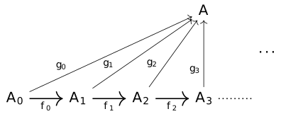
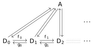
A cpo A is an upper bound of an \omega -chain of cpos in the category \mathbf {Cpo} if there is a family of continuous functions \{g_i : A_i \twoheadrightarrow A \mid i \in \mathbb {N}\} such that the following diagram commutes (i.e. g_i = g_{i+1} \circ f_i for all i \in \mathbb {N}):
DefinitionLeast upper bounds in the category \mathbf {Cpo} [dt-004S]
A cpo A is the least upper bound of an \omega -chain of cpos if is both an upper bound and if there exists a unique k for any other upper bound B such that the following diagram commutes (i.e. h_i = k \circ g_i for all i \in \mathbb {N}):
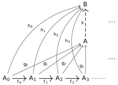
The least upper bound of such an \omega -chain is also called its colimit.
Note: Uniqueness of lubs is up to isomorphism. That is, if A and B are both colimits of our \omega -chain, then A \simeq B.
DefinitionEndofunctors on \textbf {Cpo} [dt-004T]
An endofunctor on the category \textbf {Cpo} is a functor \textbf {Cpo} \rightarrow \textbf {Cpo}, i.e. a mapping \mathcal {F} on cpos together with a mapping \mathcal {F} on continuous functions, such that:
- If f : A \twoheadrightarrow B then \mathcal {F}(f) : \mathcal {F}(A)\twoheadrightarrow \mathcal {F}(B)
- \mathcal {F}(\mathsf {id}_A : A\twoheadrightarrow A) = \mathsf {id}_{\mathcal {F}(A)} : \mathcal {F}(A)\twoheadrightarrow \mathcal {F}(A)
- \mathcal {F}(f \circ g) = \mathcal {F}(f) \circ \mathcal {F}(g)
Remark [dt-004U]
Observe that, given the information ordering for cpos where A \sqsubseteq B if there exists a continuous function A \twoheadrightarrow B, the functor laws necessarily imply monotonicity for all endofunctors \mathcal {F}.
DefinitionCocontinuous endofunctors [dt-004V]
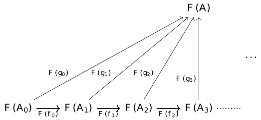
An endofunctor \mathcal {F} is cocontinuous iff it preserves colimits of \omega -chains of cpos. That is, given a chain where A is a colimit:
DefinitionFixed points of endofunctors on \mathbf {Cpo} [dt-004W]
A fixed point of an endofunctor on cpos \mathcal {F} is a cpo \mathcal {F} such that \mathcal {F}(A) \simeq A.
Note.
In Scott's approach, which we follow here, our fixed points are up to isomorphism (suitable for languages with isorecursive types), but there are other approaches where they are equalities (suitable for languages with equirecursive types).
TheoremFixed point theorem for endofunctors on \mathbf {Cpo} [dt-004X]
Every cocontinuous endofunctor \mathcal {F} on cpos has a least fixed point, given by the colimit of the \omega -chain:

ExampleBinary Numbers [dt-004Y]
Consider the Haskell-style data type: \textbf {data}\ \mathit {Bin} = \mathsf {Zero}\ \mathit {Bin} \mid \mathsf {Empty} \mid \mathsf {One}\ \mathit {Bin} So, e.g. \mathsf {One}\ (\mathsf {Zero}\ (\mathsf {One}\ \mathsf {Empty})) : \mathit {Bin}.
The recursive domain equation is, expressed as a fixed point: B \simeq \mathcal {F}(B)\quad \text {where}\ \mathcal {F}(X) = X + \mathbf {1} + X We wish to show that \mathcal {F} is a cocontinuous endofunctor.
We have a mapping \mathcal {F} on cpos (objects of the category \textbf {Cpo}), but for it to be a functor we additionally need a mapping \mathcal {F} on continuous functions (morphisms of the category \textbf {Cpo}).
Recalling our sum construction, we may remember that sums are already a bifunctor \textbf {Cpo} \times \textbf {Cpo} \rightarrow \textbf {Cpo} (Theorem [dt-0038]). Thus, our mapping on continuous functions \mathcal {F} can be derived from our mapping on cpos \mathcal {F} by using the morphism mapping from the sum construction (Definition [dt-0037]). Given a continuous function f : A \twoheadrightarrow B, our morphism mapping is:
\begin {array}{l} \mathcal {F}(f) : \mathcal {F}(A)\twoheadrightarrow \mathcal {F}(B)\\ \mathcal {F}(f) \triangleq f + \mathsf {id}_\textbf {1} + f \end {array}Proof that this endofunctor is cocontinuous is left for the reader. Hence the semantics of the type \mathit {Bin}, i.e. \llbracket \mathit {Bin} \rrbracket : \textbf {Cpo} is the least fixed point of \mathcal {F}, i.e. the colimit of the \omega -chain:

Let us visualise this chain. Here the sum injections have been written as \textsf {Z, E, O} rather than (combinations of) \textsf {inl} and \textsf {inr} to keep the connection with the Haskell data type clear.
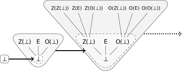
Thus, the nth cpo in the chain contains binary numbers with at most n defined digits. The colimit of the chain contains all binary numbers (finite, partial, and infinite!).
Exercise [dt-005M]
Show that \mathcal {F}(X) \triangleq \mathbf {1} + X and \mathcal {F}(f) \triangleq \mathsf {id}_\mathbf {1} + f (using our + operator for functions) define an endofunctor \mathbf {Cpo} \rightarrow \mathbf {Cpo}, i.e. that they satisfy the functor laws.
Solution.
- We must show \mathcal {F}(\mathsf {id}_A : A \twoheadrightarrow A) = \mathsf {id}_{\mathcal {F}(A)} : \mathcal {F}(A) \twoheadrightarrow \mathcal {F}(A). \begin {array}{lcl} \mathcal {F}(\mathsf {id}_A)& =& \mathsf {id}_\mathbf {1} + \mathsf {id}_A\\ &=& \mathsf {id}_{\mathbf {1} + A}\\ &=& \mathsf {id}_{\mathcal {F}(A)} \end {array}
- We must show \mathcal {F}(f \circ g) = \mathcal {F}(f) \circ \mathcal {F}(g). \begin {array}{lcl} \mathcal {F}(f \circ g) &=& \mathsf {id}_\mathbf {1} + (f \circ g) \\ &=& (\mathsf {id}_\mathbf {1} + f) \circ (\mathsf {id}_\mathbf {1} + g) \\ & = & \mathcal {F}(f) \circ \mathcal {F}(g) \end {array}
Constructing endofunctors [dt-0050]
If we have a mapping on cpos \mathcal {F} : \textbf {Cpo} \rightarrow \textbf {Cpo} that is made up of the primitives \times , +, \otimes , \oplus , \mathbf {1} and (\cdot )_\bot , we can generate a corresponding morphism mapping on continuous functions \mathcal {F} : (A\twoheadrightarrow B) \rightarrow (\mathcal {F}(A)\twoheadrightarrow \mathcal {F}(B)) by using the corresponding morphism mappings of each of these operators. Thus any such mapping can be turned into an endofunctor.
ExampleMaking endofunctors for algebraic data types [dt-0051]
\begin {array}{llr} \textsf {Object mapping} & \textsf {Morphism mapping}\\[0.2em] \mathcal {F}(X) = X + \mathbf {1} & \mathcal {F}(f) = f + \mathsf {id}_\mathbf {1} & \quad \quad \text {((co)-natural numbers)} \\ \mathcal {F}(X) = \mathbf {1} + (\mathbb {Z}_\bot \times X) & \mathcal {F}(f) = \mathsf {id}_\mathbf {1} + (\mathsf {id}_{\mathbb {Z}_\bot } \times f) & \text {((co)-lists of integers)}\\ \end {array}
Exercise [dt-005N]
The lazy natural numbers, also called conats, are defined as the least solution to the equation X \simeq \mathbf {1} + X.
- Sketch the first four approximations to the least fixed point. Call the two sum injections \mathsf {zero} and \mathsf {succ}.
Solution.
\begin {array}{lcl} A_0 & = & \{\bot \} \\ A_1 & = & \{\mathsf {zero}\ \bot , \mathsf {succ}\ \bot , \bot \} \\ A_2 & = & \{\mathsf {zero}\ \bot , \mathsf {succ}\ \bot , \mathsf {succ}\ (\mathsf {zero}\ \bot ), \mathsf {succ}\ (\mathsf {succ}\ \bot ), \bot \} \\ A_3 & = & \{\mathsf {zero}\ \bot , \mathsf {succ}\ \bot , \mathsf {succ}\ (\mathsf {zero}\ \bot ), \mathsf {succ}\ (\mathsf {succ}\ \bot ), \mathsf {succ}\ (\mathsf {succ}\ (\mathsf {zero}\ \bot )), \mathsf {succ}\ (\mathsf {succ}\ (\mathsf {succ}\ \bot )), \bot \} \\ \end {array} - Repeat this exercise assuming:
- \mathsf {zero} is strict (i.e. \mathsf {zero}\ \bot = \bot )
Solution.
\begin {array}{lcl} A_0 & = & \{\bot \} \\ A_1 & = & \{\mathsf {succ}\ \bot , \bot \} \\ A_2 & = & \{\mathsf {succ}\ \bot , \mathsf {succ}\ (\mathsf {succ}\ \bot ), \bot \} \\ A_3 & = & \{\mathsf {succ}\ \bot , \mathsf {succ}\ (\mathsf {succ}\ \bot ), \mathsf {succ}\ (\mathsf {succ}\ (\mathsf {succ}\ \bot )), \bot \} \\ \end {array} - \mathsf {succ} is strict (i.e. \mathsf {succ}\ \bot = \bot )
Solution.
\begin {array}{lcl} A_0 & = & \{\bot \} \\ A_1 & = & \{\mathsf {zero}\ \bot , \bot \} \\ A_2 & = & \{\mathsf {zero}\ \bot , \mathsf {succ}\ (\mathsf {zero}\ \bot ), \bot \} \\ A_3 & = & \{\mathsf {zero}\ \bot , \mathsf {succ}\ (\mathsf {zero}\ \bot ), \mathsf {succ}\ (\mathsf {succ}\ (\mathsf {zero}\ \bot )), \bot \} \\ \end {array}
- \mathsf {zero} is strict (i.e. \mathsf {zero}\ \bot = \bot )
From \textbf {Cpo} to \textbf {Cpo}^{\textbf {R}} [dt-0052]
ProblemContravariance in the function arrow [dt-0053]
We cannot get morphism mappings in the category \textbf {Cpo} as easily as § [dt-0050] when our object mapping makes use of the function operators \mathbin {\circ \hspace{-0.4em}\twoheadrightarrow } and \twoheadrightarrow , as they are contravariant in their first argument. This means the functor that they extend to is not \textbf {Cpo} \rightarrow \textbf {Cpo} but \textbf {Cpo}^\textsf {op} \rightarrow \textbf {Cpo}, where \textbf {Cpo}^\textsf {op} is the dual category of \textbf {Cpo}. The morphisms end up the wrong way around.
As an example, consider \mathcal {F}(X) = X\twoheadrightarrow \mathbb {Z}_\bot . Then, recalling the morphism mapping of the \twoheadrightarrow functor: \dfrac {f : A \twoheadrightarrow B \quad g : C\twoheadrightarrow D}{f\twoheadrightarrow g : (B\twoheadrightarrow C)\twoheadrightarrow (A\twoheadrightarrow D)} We can generate a morphism mapping for \mathcal {F}: \mathcal {F}(f)\; =\; f\twoheadrightarrow \mathsf {id}_{\mathbb {Z}_\bot }\; =\; (\lambda h.\ \mathsf {id}_{\mathbb {Z}_\bot }\circ h \circ f)\; = \;(\lambda h.\ h \circ f) However, this mapping has the wrong type. For f : A\twoheadrightarrow B, then \mathcal {F}(f) : (B\twoheadrightarrow \mathbb {Z}_\bot ) \rightarrow (A\twoheadrightarrow \mathbb {Z}_\bot ), which is \mathcal {F}(B)\twoheadrightarrow \mathcal {F}(A), not the required \mathcal {F}(A)\twoheadrightarrow \mathcal {F}(B). This is because the generated functor is contravariant, not covariant.
Exercise [dt-005O]
Show that, in contrast to \mathcal {F}(X) = X\twoheadrightarrow \mathbb {Z}_\bot from Problem [dt-0053], the mapping \mathcal {G}(X) = \mathbb {Z}_\bot \twoheadrightarrow X can be extended to continuous functions giving a covariant endofunctor on \textbf {Cpo}.
Given a continuous function f : A \twoheadrightarrow B, we must produce a continuous function \mathcal {F}(f) : (\mathbb {Z}_\bot \twoheadrightarrow A) \twoheadrightarrow (\mathbb {Z}_\bot \twoheadrightarrow B), defined as follows:
\mathcal {F}(f)(g)(x) = f \circ g(x)
Composition of continuous functions preserves continuity. The functor laws can be shown straightforwardly.
Solution.
DefinitionRetraction pair [dt-0054]
A retraction pair (f,g) on cpos A to B consists of two continuous functions A \xtofrom [g]{f} B such that:
- g \circ f = \mathsf {id}_A\quad (i.e. \forall x \in A.\ g(f(x)) = x )
- f \circ g \sqsubseteq \mathsf {id}_B\quad (i.e. \forall y \in B.\ f(g(y)) \sqsubseteq y )
Retraction pairs are weakenings of isomorphisms. Intuitively, going A \twoheadrightarrow B\twoheadrightarrow A, all information is preserved due to requirement 1, but going B\twoheadrightarrow A\twoheadrightarrow B, we may lose some information (hence the use of \sqsubseteq in requirement 2).
ExampleExamples and counterexamples of retraction pairs [dt-0055]
Here are two examples of retraction pairs:
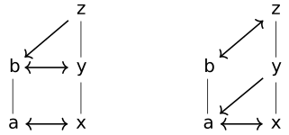
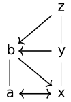
The following, however, are not retraction pairs A \xtofrom [g]{f} B:
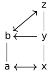
(y \mapsto b \mapsto z but z \not \sqsubseteq y)
(b \mapsto x \mapsto a but a \neq b)
DefinitionComposition of retraction pairs [dt-0056]
We can compose retraction pairs by composing their embedding and projection:

CorollaryDerived products of retraction pairs [dt-0057]
It follows from the definition of retraction pairs that, for a pair \xtofrom [g]{f}:
- f and g are strict, i.e. f(\bot ) = \bot and g(\bot ) = \bot .
- g is uniquely determined by f and vice-versa, so if another retraction pair \xtofrom [g']{f} exists, then g = g'. To see why, remember that f and g must be continuous and therefore monotonic.
- A is isomorphic to the range of f, i.e. A \simeq \{ f(x) \mid x \in A\} \subseteq B.
DefinitionThe category \textbf {Cpo}^\textbf {R} [dt-0058]
The category \textbf {Cpo}^\textbf {R} is the category where the objects are cpos, the morphisms are retraction pairs, composition is as in Definition [dt-0056] and identity is just the retraction pair A \xtofrom [\lambda x. x]{\lambda x. x} A.
DefinitionInformation ordering in \textbf {Cpo}^\textbf {R} [dt-0059]
The third point in Corollary [dt-0057] suggests a notion of approximation, or information ordering, for cpos. Rather than say, as we did in § [dt-004O], that for cpos A and B, A \sqsubseteq B iff there exists a continuous function A\twoheadrightarrow B, we now say:
Generalising to \textbf {Cpo}^\textbf {R} [dt-005A]
All of our other notions for \textbf {Cpo} naturally generalise to a setting with retraction pairs \textbf {Cpo}^\textbf {R}: least elements, \omega -chains, upper bounds, colimits, cocontinuous endofunctors and so on.
Definition\omega -chains of cpos in the category \mathbf {Cpo}^\textbf {R} [dt-005C]
An \omega -chain of cpos in the category \mathbf {Cpo}^\textbf {R} consists of a family of cpos \{D_i \mid i \in \mathbb {N} \}, together with a family of retraction pairs D_i \xtofrom [g_i]{f_i} D_{i+1}, shown below:

DefinitionEndofunctors on \textbf {Cpo}^\textbf {R} [dt-005D]
An endofunctor on the category \textbf {Cpo}^\textbf {R} is a functor \textbf {Cpo}^\textbf {R} \rightarrow \textbf {Cpo}^\textbf {R}, i.e. a mapping \mathcal {F} on cpos together with a mapping \mathcal {F} on retraction pairs, such that:
- If (f,g) is a retraction pair A \xtofrom [g]{f} B then \mathcal {F}(f,g) is a retraction pair \mathcal {F}(A)\xtofrom []{} \mathcal {F}(B)
- \mathcal {F}(\mathsf {id}_A : A\xtofrom []{} A) = \mathsf {id}_{\mathcal {F}(A)} : \mathcal {F}(A)\xtofrom []{} \mathcal {F}(A)
- \mathcal {F}(f \circ g) = \mathcal {F}(f) \circ \mathcal {F}(g) (where \circ is composition of retraction pairs)
DefinitionUpper bounds in the category \mathbf {Cpo}^\mathbf {R} [dt-005G]
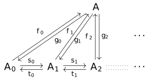
A cpo A is an upper bound of an \omega -chain of cpos A_i in the category \mathbf {Cpo}^\textbf {R} if there is a family of retraction pairs A_i \xtofrom [g_i]{f_i} A such that the following diagram commutes (i.e. for all i \in \mathbb {N}, (f_i, g_i) = (f_{i+1},g_{i+1}) \circ (s_i,t_i), where \circ is composition of retraction pairs):
DefinitionColimits in the category \mathbf {Cpo}^\mathbf {R} [dt-005F]
A cpo A is the colimit of an \omega -chain of cpos A_i if is both an upper bound, i.e. there exists retraction pairs (f_i,g_i) : A_i \xtofrom []{} A, and for any other upper bound B, for which there will exist retraction pairs (m_i,n_i) : A_i \xtofrom []{} B, there exists a unique retraction pair A \xtofrom [k']{k} B such that (m_i,n_i) = (k,k') \circ (f_i,g_i) for all i \in \mathbb {N}, where \circ is composition of retraction pairs. Viewed diagramatically, it is the same as Definition [dt-004S] where continuous functions are replaced by retraction pairs.
DefinitionCocontinuous endofunctors on \textbf {Cpo}^\textbf {R} [dt-005E]
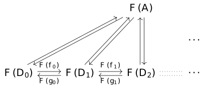
An endofunctor \mathcal {F} is cocontinuous iff it preserves colimits of \omega -chains of cpos. That is, given a chain where A is a colimit:
Extending cpo Mappings to endofunctors on \textbf {Cpo}^\mathbf {R} [dt-005I]
If \mathcal {F} is a mapping on cpos built up from basic cpos using the constructions \times , \otimes , +, \oplus , (\cdot )_\bot , as well as \twoheadrightarrow and \mathbin {\circ \hspace{-0.4em}\twoheadrightarrow }, then \mathcal {F} extends to a (covariant!) cocontinuous functor on \textbf {Cpo}^\mathbf {R}. We shall detail the construction for products and functions here, but the other constructions are all similar.
Definition\times operation for retraction pairs [dt-005J]
Given two retraction pairs (f,g) and (h,i), our retraction pair for their product is just the product of their embedding and projection, i.e. (f \times h, g \times i), using our product operation on continuous functions: \dfrac {A \xtofrom [g]{f} B\quad C \xtofrom [i]{h} D}{A\times C \xtofrom [g \times i]{f \times h} B \times D}
Definition\twoheadrightarrow operation for retraction pairs [dt-005K]
We are given two retraction pairs A \xtofrom [g]{f} B and C \xtofrom [i]{h} D. To define a suitable covariant functor, we define our morphism mapping in terms of our \twoheadrightarrow operation on continuous functions: (f,g) \twoheadrightarrow (h,i) \; \triangleq \; (g\twoheadrightarrow h, f \twoheadrightarrow i) Note that the positions of f and g are swapped in the above definition. \dfrac {A \xtofrom [g]{f} B \quad C \xtofrom [i]{h} D}{A \twoheadrightarrow C \xtofrom [f \twoheadrightarrow i]{g \twoheadrightarrow h} B \twoheadrightarrow D} Unlike with the category \textbf {Cpo}, this functor is not contravariant but covariant: Note the positions of A and B are not swapped!
TheoremFixed point theorem for endofunctors on \textbf {Cpo}^\textbf {R} [dt-005B]
Every cocontinuous endofunctor \mathcal {F} on \mathbf {Cpo}^\textbf {R} has a least fixed point, given by the colimit of the ascending \omega -chain:

ConstructionThe colimit D^\infty [dt-005H]
Given an \omega -chain:
The colimit (or inverse limit) is the cpo of \omega -tuples: D_\infty \; \triangleq \; \left \{ (x_0, x_1, \dots ) \mid x_i \in D_i \land x_i = g_i(x_{i+1}) \right \} That is, it is countable sequence of elements, one for each domain D_i, where each element is consistent with earlier elements.
Ordering: The ordering is the pointwise ordering of products, naturally generalised to \omega -tuples. Under this ordering, D_\infty is a cpo. In fact if each D_i is a Scott domain, so is D_\infty .
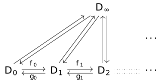
We shall prove that D_\infty is an upper bound of the \omega -chain. Proof that it is the least upper bound is straightforward but tedious, and is omitted. We must construct a family of retraction pairs:
\left \{ D_i \xtofrom [\theta _{\infty ,i}]{\theta _{i,\infty }} D_\infty \middle |\;\; i \in \mathbb {N}\;\; \right \}
such that the following diagram commutes:
Proof.
Semantics of untyped \lambda -calculus [dt-005L]
Recall the untyped \lambda calculus:
Untyped \lambda -calculus consists only of untyped (higher-order) functions:
e \; \Coloneqq \; x \mid \lambda x. e \mid e_1\ e_2
DefinitionUntyped \lambda -calculus [dt-004K]


We will now sketch a proof of the retraction pair between D_\infty and D_\infty \twoheadrightarrow D_\infty , by providing two functions, \textbf {\textsf {up}} : D_\infty \rightarrow (D_\infty \twoheadrightarrow D_\infty ) and its inverse \textbf {\textsf {down}} : (D_\infty \twoheadrightarrow D_\infty ) \rightarrow D_\infty .
Observe that each element of D_i (for i > 0) is a function D_{i-1} \twoheadrightarrow D_{i-1}. Therefore, an element of the colimit D_\infty is an \omega -tuple of such functions. To define \textbf {\textsf {up}}(d)(x), we must essentially "apply" each function in the element d \in D_\infty (viewed as an \omega -tuple of functions) to the element x \in D_\infty (viewed as an \omega -tuple of values). More specifically, we say that \textbf {\textsf {up}}(d)(x) is an \omega -tuple (y_m \mid y \in \mathbb {N}), as follows: y_m = \bigsqcup _{k \in \mathbb {N}} \theta _{m+k,m}(d_{m+k+1}(x_{m+k})) To define \textbf {\textsf {down}}(f), we are given a (continuous) function f : D_\infty \twoheadrightarrow D_\infty and must construct the \omega -tuple of approximations at every D_n. We do this by projecting the action of f down to D_n. We say that \textbf {\textsf {down}}(f) is an \omega -tuple (v_n \mid n \in \mathbb {N}) where: \begin {array}{lcl} v_0 & \triangleq & \theta _{\infty ,0}(f(\theta _{0,\infty }(\bot _{D_0})))\\ v_{n+1} & \triangleq & \theta _{\infty ,n} \circ f \circ \theta _{n,\infty } \end {array}
DefinitionDenotations for untyped \lambda -calculus
Using the new functions \textbf {\textsf {up}} and \textbf {\textsf {down}}, it is now straightforward to define a semantics for untyped \lambda -calculus, where \sigma is an environment \mathsf {Var} \rightarrow D_\infty : \llbracket \cdot \rrbracket : (\mathsf {Var} \rightarrow D_\infty )\twoheadrightarrow D_\infty \begin {array}{lcl} \llbracket x \rrbracket \sigma & = & \sigma (x) \\ \llbracket e_0\ e_1 \rrbracket \sigma & = & \textbf {\textsf {up}}(\llbracket e_0 \rrbracket \sigma ) (\llbracket e_1 \rrbracket \sigma )\\ \llbracket \lambda x.\ e \rrbracket \sigma & = & \textbf {\textsf {down}}(\boldsymbol {\lambda } v \in D_{\infty }.\ \llbracket e \rrbracket \ \sigma (x \mapsto v) ) \end {array} This semantics does not distinguish non-terminating computations from terminating ones. To model call-by-value more faithfully, we could use the equation D \simeq D\twoheadrightarrow D_\bot instead, and for call-by-name we could use D \simeq D_\bot \twoheadrightarrow D_\bot . The constructions are very similar.