Lecture Notes. Domain theory [dt-001Y]
These lecture notes are based on the material I used to teach the Domain Theory (TypeSIG) course at the University of Edinburgh in 2024.
LectureSemantics and recursion [dt-0005]
This lecture is based on material from Graham Hutton, Dana Scott, Joseph Stoy, Carl Gunter, and Glynn Winskel.
Denotational semantics [dt-0003]
In this course we are concerned with programming languages, which, as with natural languages, consist of a syntax and semantics. The syntax of a language is, for our purposes, merely an inductively-defined tree structure (i.e. abstract syntax).
DefinitionThe \mathcal {C} Language (without loops) [dt-0000]
Using notation similar to Backus-Naur Form (BNF): \begin {array}{lcl} \mathcal {E} & \Coloneqq & n \mid x \mid \mathcal {E}_1 + \mathcal {E}_2 \mid \mathcal {E}_1 - \mathcal {E}_2\\ \mathcal {B} & \Coloneqq & \mathsf {false} \mid \mathsf {true} \mid \neg \mathcal {B} \mid \mathcal {E}_1 = \mathcal {E}_2\\ \mathcal {C} & \Coloneqq & \mathsf {skip} \mid x := \mathcal {E} \mid \mathcal {C}_1 ; \mathcal {C}_2 \mid \mathsf {if}\ \mathcal {B}\ \mathsf {then}\ \mathcal {C}_1\ \mathsf {else}\ \mathcal {C}_2\\ x & \in & \mathcal {V}\; \textit {(variables)}\\ n & \in & \mathbb {N} \end {array}
In the language above, there are three syntactic classes: \mathcal {E}, \mathcal {B}, and \mathcal {C}.
DefinitionDenotational semantics [dt-0001]
A denotational semantics consists of, for each syntactic class \mathcal {X} in a language:
- A semantic domain D which can be any set of mathematical objects (although, as we will see later, it is helpful if it obeys certain properties).
- A valuation function \llbracket \cdot \rrbracket : \mathcal {X} \rightarrow D. We require that this function be a homomorphism, that is that it is compositional. This means that the valuation (or denotation) of an expression should be made from the denotation of its components. In other words, for each syntactic constructor C(e_1,e_2,\dots ), we should have a mathematical operation f(x_1,x_2,\dots ) such that the denotation of C can be defined as: \llbracket C(e_1, e_2, \dots ) \rrbracket = f(\llbracket e_1 \rrbracket , \llbracket e_2 \rrbracket , \dots )
Remark [dt-0002]
The choices of semantic domain and valuation function are, essentially, arbitrary: we choose objects that reflect those aspects of our programs that we are interested in. For most of the simple languages we will examine, we are only concerned with the results of the computation, which is a semantics suitable for reasoning about program behaviour and correctness. However, there also exist denotational cost models that compositionally assign a measure of program performance to syntax. This measure is just another kind of denotational semantics.
ExampleDenotational semantics for the \mathcal {C} language (without loops) [dt-0004]
We shall first select a semantic domain for each syntactic class: \begin {array}{lcl} \mathbf {E} & \triangleq & \Sigma \rightarrow \mathbb {Z} \\ \mathbf {B} & \triangleq & \Sigma \rightarrow \mathbb {B} \\ \mathbf {C} & \triangleq & \Sigma \rightarrow \Sigma \\ \end {array} Here, \Sigma represents the set of states, which contains the values assigned to all variables: \Sigma \;\triangleq \; \mathcal {V} \rightarrow \mathbb {Z}
Now, we define our valuation functions, \llbracket \cdot \rrbracket _\mathcal {E} : \mathcal {E} \rightarrow \mathbf {E} : \begin {array}{lcl} \llbracket n \rrbracket _\mathcal {E}\ \sigma & = & n \\ \llbracket x \rrbracket _\mathcal {E}\ \sigma & = & \sigma (x) \\ \llbracket e_1 + e_2 \rrbracket _\mathcal {E}\ \sigma & = & \llbracket e_1 \rrbracket _\mathcal {E}\ \sigma + \llbracket e_2 \rrbracket _\mathcal {E}\ \sigma \\ \llbracket e_1 - e_2 \rrbracket _\mathcal {E}\ \sigma & = & \llbracket e_1 \rrbracket _\mathcal {E}\ \sigma - \llbracket e_2 \rrbracket _\mathcal {E}\ \sigma \\[2em] \end {array} and \llbracket \cdot \rrbracket _\mathcal {B} : \mathcal {B} \rightarrow \mathbf {B}: \begin {array}{lcl} \llbracket \mathsf {false} \rrbracket _\mathcal {B}\ \sigma & = & \mathit {F} \\ \llbracket \mathsf {true} \rrbracket _\mathcal {B}\ \sigma & = & \mathit {T} \\ \llbracket \neg b \rrbracket _\mathcal {B}\ \sigma & = & \begin {cases}\mathit {F} & \text {if}\ \llbracket b \rrbracket _\mathcal {B}\ \sigma = \mathit {T} \\ \mathit {T} & \text {otherwise} \end {cases} \\[1.1em] \llbracket e_1 = e_2 \rrbracket _\mathcal {B}\ \sigma & = & \begin {cases}\mathit {T} & \text {if}\ \llbracket e_1 \rrbracket _\mathcal {E}\ \sigma = \llbracket e_2 \rrbracket _\mathcal {E}\ \sigma \\ \mathit {F} & \text {otherwise} \end {cases} \end {array} and \llbracket \cdot \rrbracket _\mathcal {C} : \mathcal {C} \rightarrow \mathbf {C}: \begin {array}{lcl} \llbracket \mathsf {skip} \rrbracket _\mathcal {C}\ \sigma & = & \sigma \\ \llbracket x := e \rrbracket _\mathcal {C}\ \sigma & = & \sigma \left (x \mapsto \llbracket e \rrbracket _\mathcal {E}\right ) \\ \llbracket c_1 ; c_2 \rrbracket _\mathcal {C}\ \sigma & = & \llbracket c_2 \rrbracket _\mathcal {C}\ \left (\llbracket c_1 \rrbracket _\mathcal {C}\ \sigma \right ) \\[0.3em] \llbracket \textsf {if}\ b\ \textsf {then}\ c_1\ \textsf {else}\ c_2 \rrbracket _\mathcal {C}\ \sigma & = & \begin {cases}\llbracket c_1 \rrbracket _\mathcal {C}\ \sigma & \text {if}\ \llbracket b \rrbracket _\mathcal {B}\ \sigma = \mathit {T} \\ \llbracket c_2 \rrbracket _\mathcal {C}\ \sigma & \text {otherwise} \end {cases} \end {array}
Recursion [dt-000L]
So far, our semantic domains have just been (functions of) sets. While these have the advantage of being mathematically simple and intuitive, two language features make these sets insufficient for our purposes:
- Recursively defined programs, for dealing with recursion and loops, and
- Recursively defined semantic domains, for dealing with higher-order programs.
Recursively defined programs [dt-0006]
Suppose we extended the \mathcal {C} language with a while loop construct: \mathcal {C}\; \Coloneqq \; \cdots \mid \mathsf {while}\ \mathcal {B}\ \mathsf {do}\ \mathcal {C}\ \mathsf {od} The intuitive way to assign a semantics would be to use a recursive function: \llbracket \mathsf {while}\ b\ \mathsf {do}\ c\ \mathsf {od} \rrbracket _\mathcal {C}\ \sigma \; = \; \begin {cases} \llbracket \mathsf {while}\ b\ \mathsf {do}\ c\ \mathsf {od} \rrbracket _\mathcal {C}\ (\llbracket c \rrbracket _\mathcal {C}\ \sigma ) & \text {if}\ \llbracket b \rrbracket _\mathcal {B}\ \sigma = \mathit {T} \\ \sigma & \text {otherwise} \end {cases} However, such an equation is not a good definition. If we consider the trivial infinite loop program L \triangleq \mathsf {while}\ \mathsf {true}\ \mathsf {do}\ \mathsf {skip}\ \mathsf {od}, and compute its semantics, we end up with: \llbracket \mathsf {while}\ \mathsf {true}\ \mathsf {do}\ \mathsf {skip}\ \mathsf {od} \rrbracket _\mathcal {C}\ \sigma \; = \; \llbracket \mathsf {while}\ \mathsf {true}\ \mathsf {do}\ \mathsf {skip}\ \mathsf {od} \rrbracket _\mathcal {C}\ \sigma This equation is satisfied by any function \Sigma \rightarrow \Sigma , so it doesn't tell us which function corresponds to the program L.
More generally, allowing our functions to be (generally) recursive causes these issues. The loop program L gives rise to the recursive equation \ell (x) = \ell (x), which has an infinite number of solutions.
If we add recursion to our programming language, we could have programs that give rise to more complex recursive equations like f(x) = f(x) + 1. By contrast to \ell (x), f(x) has no solutions (assuming f(x) operates on integers).
Upshot.
We need an explicit notion of "non-termination" on the semantics level, to properly deal with general recursion (or iteration).
Recursively defined semantic domains [dt-0007]
Suppose we extend our notion of expressions in the \mathcal {C} language with parameterless higher-order procedures: \begin {array}{l} \mathcal {E}\; \Coloneqq \; \cdots \mid \mathsf {proc}\ \mathcal {C}\\ \mathcal {C}\; \Coloneqq \; \cdots \mid x \end {array}
ExampleUsing higher-order procedures
We can store procedures in variables, so the program: \mathit {inc} := (\mathsf {proc}\ a := a + 1); \mathit {inc}; \mathit {inc} has the same effects on the variable a as the program: a := a + 1; a := a + 1
For our denotational semantics, our domains now take this form (\textcolor {blue}{\text {blue}} parts are new vs. Example [dt-0004]), where \uplus denotes disjoint union:
\begin {array}{lcl}
\mathbf {E} & \triangleq & \Sigma \rightarrow \mathbb {Z}\textcolor {blue}{\ \uplus \ \mathbf {C}}\\
\mathbf {B} & \triangleq & \Sigma \rightarrow \mathbb {B} \\
\mathbf {C} & \triangleq & \Sigma \rightarrow \Sigma \\[0.2em]
\Sigma & \triangleq & \mathcal {V} \rightarrow \mathbb {Z}\textcolor {blue}{\ \uplus \ \mathbf {C}}
\end {array}
Give a semantics to the \mathsf {proc} construct:
Exercise [dt-000P]
Solution.
ExampleA simpler equation with no solution
Consider the recursive equation X = X \rightarrow \mathbb {B}. Cantor's theorem says that there is no set X such that X \simeq \mathcal {P}(X) (where \mathcal {P}(X) is the power set of X), and seeing as \mathcal {P}(X) \simeq (X \rightarrow \mathbb {B}) it follows that X = X \rightarrow \mathbb {B} has no solution.
Any kind of higher-order construct leads to such recursive domain equations.
Upshot.
There are no (nontrivial) set-theoretic solutions to the recursive domain equations that arise from higher-order language constructs.
We will return to this problem later on! For now, let's focus on representing non-termination.
Flat domains and information ordering [dt-0009]
The bottom value [dt-000A]
Following Scott, we introduce a special bottom value \bot to our semantic domains. \bot \ \text {represents}\ \begin {cases}\text {an undefined value;}\\\text {an error value;}\\\text {a \emph {non-terminating} computation.} \end {cases}
DefinitionFlat domain [dt-0008]
Given a set X, the flat domain (or lifted set) X_\bot is just the set X \cup \{ \bot \} (where \bot \notin X).
DefinitionInformation ordering [dt-000B]
An information ordering is a partial order on denotations, written a \sqsubseteq b. This indicates that b is approximated by, or carries more information than, or is more well-defined than a. Naturally, the bottom value, being totally uninformative, is always the least element in this ordering.
ExampleInformation ordering for flat domains [dt-000C]
Consider a flat domain X_\bot . There is a natural information ordering \sqsubseteq on X_\bot :
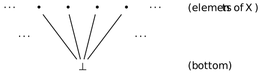
Formally, we say x \sqsubseteq y iff (x = y \lor x = \bot ).
Warning.
Don't confuse the information ordering on numbers, i.e. \sqsubseteq on \mathbb {Z}_\bot , with the numerical ordering \leq on \mathbb {Z}. We know 0 \leq 1, but 0 and 1 are not comparable in our flat information ordering.
Combining domains [dt-000D]
Some of our semantics may depend on the combination of multiple domains, i.e. semantic functions of multiple arguments. As an example, the semantics of an \mathsf {if} statement combines the semantics of the condition and the semantics of each of the two branches. In such scenarios, our domains are no longer flat — we must generalise to pointed posets.
DefinitionPointed poset [dt-000G]
A pointed poset is a partially ordered set with a bottom value.
ConstructionProduct of two pointed posets [dt-000E]
Given two pointed posets X and Y, the product poset X \times Y is ordered as follows: (x,y) \sqsubseteq _{X \times Y} (x',y') \quad \text {iff} \quad x \sqsubseteq _X x' \land y \sqsubseteq _Y y' Intuitively, this says that "the information content of a pair of values is increased by increasing the information of either or both of its component values".
This product poset is also pointed, with bottom value \bot _{X \times Y} being (\bot _A, \bot _B).
ExampleThe domain \mathbb {B}_\bot \times \mathbb {B}_\bot [dt-000F]
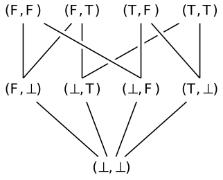
As can be seen above, the domain \mathbb {B}_\bot \times \mathbb {B}_\bot is not flat, but it is still a pointed poset.
Monotonic functions [dt-000H]
If we model our semantic domains for values with pointed posets, then programs are modelled by functions between such posets. But, not all functions are suitable:
ExampleThe halting query [dt-000I]
The function H : \mathbb {B}_\bot \rightarrow \mathbb {B}_\bot seems to let us solve the halting problem, assuming \bot represents non-termination: H(v) \; = \; \begin {cases} F & \text {if}\ v = \bot \\ T & \text {otherwise} \end {cases}
It stands to reason that the amount of information we get out of our functions should grow as we increase the amount of information we put into them. Such functions are called monotonic with respect to our information ordering.
DefinitionMonotonicity [dt-000J]
A function f : X \rightarrow Y between posets X and Y is monotone (or monotonic) if, for all x, y \in X: x \sqsubseteq y\; \text {implies}\; f(x) \sqsubseteq f(y)
DefinitionStrictness [dt-000K]
A function f : X \rightarrow Y on pointed posets X and Y is strict if it preserves the bottom value, i.e. f(\bot _X) = \bot _Y.
Thesis.
Computable functions are monotonic (observe that H is not).
Exercise [dt-000N]
Consider the functions \mathbb {B}_\bot \rightarrow \mathbb {B}_\bot . Which ones are monotonic? There are a total of 27 such functions but only three significant classes.
Solution.
Exercise [dt-000O]
Let \mathbf {K}_K denote the chain of values x_1, x_2, x_3, \dots , x_K where a \leq b implies x_a \sqsubseteq x_b. There is one monotonic function \mathbf {K}_1 \rightarrow \mathbf {K}_1:

And there are three monotonic functions \mathbf {K}_2 \rightarrow \mathbf {K}_2:
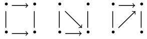
- Write down the monotonic functions \mathbf {K}_3 \rightarrow \mathbf {K}_3.
- Write a simple recursive program to calculate the number of monotonic functions \mathbf {K}_n \rightarrow \mathbf {K}_m.
Solution.
When drawn as a diagram like the above, the monotonic functions are all those whose lines do not cross.
Solution.
In Haskell:
monotonics :: Int -> Int -> Int
monotonics n 1 = 1
monotonics n m = sum [monotonics (n-x) (m-1) | x <- [0..n]]
Fixed points [dt-000U]
From recursion to fixed points [dt-000R]
Consider our recursive \mathsf {while} loop semantics from § [dt-0006]: \llbracket \mathsf {while}\ b\ \mathsf {do}\ c\ \mathsf {od} \rrbracket _\mathcal {C}\ \sigma \; = \; \begin {cases} \llbracket \mathsf {while}\ b\ \mathsf {do}\ c\ \mathsf {od} \rrbracket _\mathcal {C}\ (\llbracket c \rrbracket _\mathcal {C}\ \sigma ) & \text {if}\ \llbracket b \rrbracket _\mathcal {B}\ \sigma = \mathit {T} \\ \sigma & \text {otherwise} \end {cases} How do we ensure that solutions exist for such recursive equations? And, if multiple solutions exist, how do we decide which one to pick? To address these questions, let's factor out everything in our definition except the recursion into a separate (higher-order) function: \begin {array}{l} \llbracket \mathsf {while}\ b\ \mathsf {do}\ c\ \mathsf {od} \rrbracket _\mathcal {C} = f(\llbracket \mathsf {while}\ b\ \mathsf {do}\ c\ \mathsf {od} \rrbracket _\mathcal {C}) \\[0.5em] \qquad \text {where}\; f(X)\ \sigma \; \triangleq \; \begin {cases} X\ (\llbracket c \rrbracket _\mathcal {C}\ \sigma ) & \text {if}\ \llbracket b \rrbracket _\mathcal {B}\ \sigma = \mathit {T} \\ \sigma & \text {otherwise} \end {cases} \end {array} Looking at it this way, we can see that any solution to this equation must be an element of our semantic domain X \in \mathbf {C} such that f(X) = X. In other words, the problem of finding solutions to our recursive equations can be cast as the problem of finding a fixed point for non-recursive higher-order functions.
DefinitionFixed point [dt-000S]
A value x is a fixed point of a function f if f(x) = x.
Monotonicity is insufficient [dt-000T]
Exercise [dt-000Q]
- Give an example of a poset A and a monotonic function f : A \rightarrow A such that f doesn't have a fixed point.
Solution.
In the poset (\mathbb {N},\leq ), the function f(x) = x + 1 has no fixed points.
- Give an example of a poset A and a monotonic function f : A \rightarrow A such that f has multiple fixed points.
Solution.
In the poset (\mathbb {N},\leq ), the function f(x) = x has infinitely many fixed points.
Problem.
Not all monotonic functions on posets have fixed points, and some have multiple fixed points!
So, requiring our functions to be monotonic is insufficient to guarantee that a single "best" solution exists.
Chains and Unfolding [dt-000Y]
- with contributions from Liam O'Connor
Intuitively, recursive programs are executed by "unfolding" as much as necessary to get a result. We would like to characterise our domains to ensure that solutions always exist, and to allow us to pick the solutions that are "minimal" in the sense that they rely on a minimal amount of unfolding.
After converting a recursive program into a non-recursive monotonic higher order function f, the fixed point we desire would intuitively be the limit of the ascending Kleene chain of f, i.e. f(f(f(f(\dots )))):
ExampleAscending Kleene chain [dt-000X]
Given a pointed poset (X,\subseteq ) and a monotonic function f : X \rightarrow X, the ascending Kleene chain is the \omega -chain: \bot \sqsubseteq f(\bot ) \sqsubseteq f(f(\bot )) \sqsubseteq f(f(f(\bot ))) \sqsubseteq \cdots Because \bot is the bottom element, we know that \bot \sqsubseteq f(\bot ). Each subsequent step in the chain exists because of monotonicity.
Each successive element of this chain is another "unfolding" of the recursion.
DefinitionChain [dt-000V]
A chain in a poset X is a totally ordered subset of X. That is, a subset Y \subseteq X is a chain iff: \forall x, y \in Y.\; x \sqsubseteq y \lor y \sqsubseteq x
Definition\omega -chain [dt-000W]
From chains to directed sets [dt-000Z]
- with contributions from Liam O'Connor
While \omega -chains are technically sufficient for denotational semantics, for our purposes it is a little more convenient to think in terms of directed sets rather than chains.
DefinitionDirected set [dt-0010]
Formally, a non-empty subset Y \subseteq X of a poset (X,\sqsubseteq ) is directed iff: \forall x, y \in Y.\ \exists z \in Y.\ x \sqsubseteq z \land y \sqsubseteq z
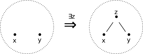
Intuitively, directed sets are "going somewhere" — given two elements we can always find a "greater" one in the set.
ExamplePower sets are directed [dt-0011]
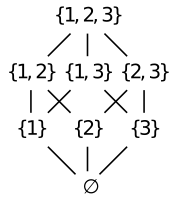
TheoremChain → Directed [dt-0012]
All non-empty chains are directed.
Proof.
Let C be a chain. Then, given two elements x,y \in C we know from totality that either x \sqsubseteq y or y \sqsubseteq x. If x \sqsubseteq y, then y is the upper bound, otherwise x is the upper bound.
DefinitionConsistent subset [dt-0013]
A subset Y \subseteq X of a poset X is consistent iff
\exists x \in X.\ \forall y \in Y.\ y \sqsubseteq x
Such an x is called an upper bound of Y.
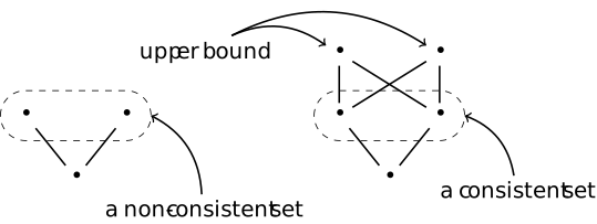
TheoremAlternative characterisation of directedness [dt-0014]
A subset Y \subseteq X of a poset X is directed iff every finite subset of Y' \subseteq Y has an upper bound in Y.
Proof.
- ⇐: Every pair of elements x,y \in Y has an upper bound simply by taking the upper bound of the set \{x,y\}.
- ⇒: Given a finite set X = \{x_1,x_2,\dots , x_n\} , we can show it has an upper bound by an inductive process, first taking the upper bound of x_1 and x_2, and then taking the upper bound of that an x_3 and so on until we have an upper bound for the whole set. This induction works because the set X is finite.
Corollary [dt-0015]
Least upper bounds [dt-0016]
DefinitionLeast upper bound [dt-0017]
Let X \subseteq Y be a subset of a poset Y. An element y \in Y is a least upper bound (or lub) for X iff:
- It is an upper bound: \forall x \in X.\ x \sqsubseteq y
- It is less than any other upper bound: \forall y' \in Y.\ (\forall x \in X. x \sqsubseteq y') \Rightarrow y \sqsubseteq y'
CorollaryProperties of \sqcup [dt-0018]
When lubs exist, the binary \sqcup operator is idempotent, commutative, and associative. Also, we have that x \sqsubseteq y iff x \sqcup y = y.
TheoremPointedness via lubs [dt-0019]
A poset Y is pointed iff \bigsqcup \emptyset exists, as the lub of an empty set is just the bottom element in the poset, i.e. \bigsqcup \emptyset = \bot .
Information intuition [dt-001A]
When the poset Y from Definition [dt-0017] is ordered by our information ordering, the intuition of the lub \bigsqcup X is that it combines all of the information content of all the elements of X but it does not add any additional information (hence least).
ExampleLubs in the domain \mathbb {B}_\bot \times \mathbb {B}_\bot [dt-001B]
- (\bot , \mathit {F}) \sqcup (\mathit {T},\bot ) = (\mathit {T},\mathit {F})
- (\bot , \mathit {F}) \sqcup (\bot ,\bot ) = (\bot ,\mathit {F})
- (\bot , \mathit {F}) \sqcup (\mathit {T}, \mathit {T}) does not exist.
Exercise [dt-001C]
Complete partial orders [dt-001E]
DefinitionComplete partial order [dt-001D]
A complete partial order or cpo (more specifically a directed complete partial order or dcpo) is a poset where lubs exist for the empty set and for all directed subsets. That is, a cpo is a poset A such that:
- A has a bottom element \bot \in A, that is the lub of the empty set, and
- \bigsqcup X exists for all directed X \subseteq A.
AsideOther kinds of completeness [dt-001F]
In Definition [dt-001D] we defined cpos in terms of directed completeness. We may consider chain completeness instead, where, rather than require lubs for every directed subset of our poset A, we require lubs for every chain X \subseteq A. We know from Theorem [dt-0012] that all chains are directed, so every directed complete cpo is also chain complete. It is also known that every chain complete cpo is also directed complete, so the notions are equivalent, although the proof is non-trivial, relying on transfinite induction (see these lecture notes for details).
If we weaken our completeness requirement to require lubs only for the countable \omega -chains and not necessarily all chains, we get what is called an \omega -cpo. All \omega -chains are chains and are therefore directed, but not all chains are \omega -chains.
Working with just \omega -cpos is common in denotational semantics practice, but working with directed completeness simplifies some of the properties we will discuss later.
Exercise [dt-001G]
For each of the following posets, determine if it is a cpo or not. If it is, describe the lubs. If it is not, give a directed set which has no lub.
- A finite pointed poset
- (\mathcal {P}(S), \subseteq ) for some set S
- (\mathbb {N},\leq )
- (\mathbb {N} \cup \{\infty \}, \leq )
- ([0,1] \subseteq \mathbb {R}, \leq )
- ([0,1) \subseteq \mathbb {R}, \leq )
- (\mathbb {Q}, \leq )
- A flat domain S_\bot for some set S.
Solution.
- A finite pointed poset is a cpo, as all directed subsets will be finite and therefore have a lub.
- (\mathcal {P}(S), \subseteq ) is a cpo as the lub is just the union.
- (\mathbb {N},\leq ) is not a cpo, as the \omega -chain 1 \leq 2 \leq 3 \leq \cdots has no lub.
- (\mathbb {N} \cup \{\infty \}, \leq ) is a cpo, as \infty is the lub of any non-repeating chain.
- ([0,1] \subseteq \mathbb {R}, \leq ) is a cpo with maximum as the lub.
- ([0,1) \subseteq \mathbb {R}, \leq ) is not a cpo, as the set \{0.9,0.99,0.999,\dots \} has a lub of 1 \notin [0,1).
- (\mathbb {Q}, \leq ) is not a cpo, and not just because it lacks a lub for \mathbb {Q} itself, but also it doesn't contain \sqrt {2}, which can be expressed as the lub of an infinite sequence of rational approximations.
- A flat domain S_\bot for some set S is a cpo, as the largest chains have two elements, and we always pick the non-\bot one as the lub.
RemarkLubs of chains [dt-001H]
The limit of the ascending Kleene chain of a monotonic function f : X \rightarrow X is the same as the least upper bound of the set \{ f^n(\bot ) \mid n \in \mathbb {N}\} (where f^n is the n-fold self-composition of the function f). If we require that our semantic domain X is a cpo, we know that this limit exists.
Our semantic domains are cpos, ensuring the presence of these limits.Thesis.
Exercise [dt-001X]
- Show that if A and B are posets and X \subseteq A \times B is directed (by the ordering in Construction [dt-000E]), then the subsets \pi _0(X) \subseteq A and \pi _1(X) \subseteq B (defined below) are also directed.
\begin {array}{lcl}
\pi _0(X) & = & \{ a \in A \mid \exists b \in B.\ (a,b) \in X \}\\
\pi _1(X) & = & \{ b \in B \mid \exists a \in A.\ (a,b) \in X \}\\
\end {array}
Solution.
Given two elements x,y \in \pi _0(X), we know that there exists b_x, b_y \in B such that (x,b_x) \in X and (y,b_y) \in X. Because X is directed, we can conclude that there exists an upper bound (z, b_z) \in X where x \sqsubseteq z and y \sqsubseteq z. As z \in \pi _0(X), z is an upper bound in \pi _0(X) for both x and y and thus \pi _0(X) is directed. The proof for \pi _1 is analogous.
- Give an example of a set X \subseteq \{\top ,\bot \}\times \{\top ,\bot \} such that \pi _0(X) and \pi _1(X) are directed, but X is not.
Solution.
X = \{(\top ,\bot ), (\bot ,\top )\} is not directed as the two elements are not comparable, but \pi _0(X) = \pi _1(X) = \{\top ,\bot \} which is directed as \bot \sqsubseteq \top .
- Show that if A and B are cpos and X \subseteq A \times B is directed, then \bigsqcup X = \left (\bigsqcup \pi _0(X), \bigsqcup \pi _1(X)\right ) Note: Together with \bot _{A\times B} = (\bot _A, \bot _B) this shows that the Cartesian product of two cpos is itself a cpo.
Solution.
Let (x,y) = \left (\bigsqcup \pi _0(X), \bigsqcup \pi _1(X)\right ). Because of the ordering in Construction [dt-000E], (x,y) is certainly a upper bound of the directed set X. To show it is the least upper bound, assume for the sake of contradiction that (x,y) is not the least upper bound of X. Then, there must be a (v,w)\sqsubset (x,y) such that \forall x \in X.\ x \sqsubseteq (v,w). But then, v would be a lesser upper bound for \pi _0(X) than x, which is supposed to be the lub. Thus there is a contradiction, and (x,y) must be the lub of X.
Continuity and Fixed Points [dt-001I]
- with contributions from Liam O'Connor
By choosing a cpo for our semantic domain, we can ensure that the Kleene chain has a limit. However, it is not guaranteed that the limit we find will be a fixed point to our monotonic function f.
ProblemMonotonicity is insufficient [dt-001K]
Consider this monotonic function g defined over a cpo (\mathbb {R} \cup \{\infty ,-\infty \}, \leq ): g(x) = \begin {cases} \tan ^{-1} x & \text {if}\ x < 0\\ 1 & \text {otherwise} \end {cases} Note this function is not continuous at 0. Starting from our \bot element -\infty , we can see that the limit of the ascending Kleene chain is 0: \begin {array}{lcl} g(-\infty ) & = & -\frac {\pi }{2}\\ g(-\frac {\pi }{2}) & = & -1\\ g(-1) & \approx & -0.78\\ \end {array} But g(0) = 1! — the lub of the Kleene chain is not a fixed point!
To address this problem, we shall strengthen our requirement on functions from mere monotonicity to continuity.
DefinitionContinuity [dt-001J]
A function f : A \rightarrow B on cpos A and B is continuous iff for all directed X \subseteq A,
- \bigsqcup \{ f(x) \mid x \in X \} exists, and
- f(\bigsqcup X) = \bigsqcup \{ f(x) \mid x \in X \}, i.e., f preserves lubs.
TheoremContinuity implies monotonicity [dt-001L]
All continuous functions are monotonic.
Consider two elements x, y of a cpo where x \sqsubseteq y. Then \{x,y\} is directed with a lub of y. By the second condition in Definition [dt-001J], we get f(y) = f(x) \sqcup f(y) which is equivalent to f(x) \sqsubseteq f(y).Proof.
ExampleMonotonic but not continuous [dt-001M]
Consider this function from \mathbb {N} \cup \{\infty \} \rightarrow \{\top ,\bot \}, defined by: f(x) = \begin {cases} \bot & \text {if}\ x \in \mathbb {N}\\ \top & \text {otherwise} \end {cases} This function is monotonic, but, taking X = \mathbb {N} (which is a directed subset of the cpo \mathbb {N} \cup \{\infty \}), then f(\bigsqcup \mathbb {N}) = f(\infty ) = \top , but \bigsqcup \{ f(n) \mid n \in \mathbb {N} \} = \bigsqcup \{ \bot \} = \bot . Thus, this function is not continuous.
Exercise [dt-001N]
Show that if a function on cpos f : A \rightarrow B is monotonic, then \bigsqcup \{ f(x) \mid x \in X \} exists for any directed X \subseteq A (i.e.the first condition for continuity in Definition [dt-001J]).
Hint: It suffices to show that \{ f(x) \mid x \in X \} \subseteq B is directed.
Solution.
Because B is a cpo, it suffices to show that \{ f(x) \mid x \in X \} \subseteq B is directed. Let a,b \in \{ f(x) \mid x \in X \}. Let x_a, x_b \in X be the values that f maps to a and b respectively, i.e. f(x_a) = a and f(x_b) = b. Because X is directed, an upper bound of x_a and x_b exists in X. Call this upper bound x_c. Because x_a \sqsubseteq x_c and x_b \sqsubseteq x_c, we know that f(x_a) = a \sqsubseteq f(x_c) and f(x_b) = b \sqsubseteq f(x_c) by monotonicity of f. Also, f(x_c) \in \{ f(x) \mid x \in X \} because x_c \in X. Therefore, because two arbitrary elements in \{ f(x) \mid x \in X \} have an upper bound within the set, the set \{ f(x) \mid x \in X \} is directed.
TheoremAlternative characterisation of continuity [dt-001O]
A function f : A \rightarrow B on cpos A and B is continuous iff:
- f is monotonic, and
- f(\bigsqcup X) = \bigsqcup \{ f(x) \mid x \in X \}, for all directed X \subseteq A
Proof.
The second condition here is identical to that of Definition [dt-001J]. The monotonicity requirement is equivalent to the first condition of Definition [dt-001J], with one direction shown by Theorem [dt-001L], and the other shown by the solution of Exercise [dt-001N].
Thesis.
Computable functions are continuous functions on cpos.
Exercise [dt-001W]
Show that if a function f : A \rightarrow B on cpos A and B is monotonic and A is finite, then f is continuous.
Hint: Finite directed sets contain their lub
Solution.
Because of Theorem [dt-001O], it suffices to show the second condition of continuity, as f is monotonic.
Because A is finite, any directed subset X \subseteq A is also finite, and therefore \bigsqcup X \in X. Because f is monotone, f(x) \sqsubseteq f (\bigsqcup X) for all x \in X.
The solution to Exercise [dt-001N] shows that \{f(x) \mid x \in X\} is directed and therefore contains its upper bound c. Because f is monotone, f(\bigsqcup X) must be c (else it would contradict the above).
Therefore \bigsqcup \{f(x) \mid x \in X\} = f (\bigsqcup X), as required.
TheoremThe Kleene fixed point theorem [dt-001P]
Let (S, \sqsubseteq ) be a cpo and f : S \rightarrow S be a continuous function. Then the lub of the Kleene chain \bigsqcup _{n\in \mathbb {N}}f^{n}(\bot ) is the least fixed point of f.
Proof.
We apply continuity to show that it is a fixed point: \begin {array}{lclr} f(\bigsqcup _{n \in \mathbb {N}} f^n(\bot ) ) & = & \bigsqcup _{n \in \mathbb {N}} f(f^n(\bot )) & \text {(continuity)} \\[0.5em] &=& \bigsqcup _{n \in \mathbb {N}} f^{n+1}(\bot )\\[0.5em] &=& \bigsqcup _{n=1,2\dots }f^{n}(\bot ) &\qquad \text {(reindexing)}\\[0.5em] &=& \bot \sqcup \bigsqcup _{n=1,2\dots }f^{n}(\bot )\\[0.5em] &=&\bigsqcup _{n\in \mathbb {N}}f^{n}(\bot )\\[0.5em] \end {array} To see that it is the least fixed point: Let y be a fixed point of f. We know that \bot \sqsubseteq y by definition of \bot . Taking f of both sides, we get f(\bot ) \sqsubseteq y. We can continue this inductively and thus we know that, for all n \in \mathbb {N}, f^n(\bot ) \sqsubseteq y. Because y is, therefore, an upper bound of the ascending Kleene chain, it must also be at least as large as the lub of that chain.
DefinitionThe \textbf {fix} operator [dt-001Q]
Let \textbf {fix}(f) denote the least fixed point of the continuous function f, that is \bigsqcup _{n\in \mathbb {N}}f^{n}(\bot ), guaranteed to exist by Theorem [dt-001P].
Exercise [dt-001S]
- What is \textbf {fix}(\mathsf {id}) where \mathsf {id} is the identity function on \mathbb {B}_\bot ?
Solution.
\bigsqcup \{ \bot , \mathsf {id}(\bot ), \mathsf {id}(\mathsf {id}(\bot )), \dots \} = \bot - What is \textbf {fix}(\kappa _\mathit {F}) where \kappa _\mathit {F} is the constant function that always returns \mathit {F}?
Solution.
\bigsqcup \{ \bot , \kappa _F(\bot ), \kappa _F(\kappa _F(\bot )), \dots \} = \mathit {F} - What is \textbf {fix}(f) where
\begin {array}{l}
f : [\mathbb {N}_\bot ] \rightarrow [\mathbb {N}_\bot ]\\
f(x) = 1::x
\end {array}
(where [\mathbb {N}_\bot ] denotes Haskell-style lazy lists of \mathbb {N}_\bot )?
Solution.
\bigsqcup \{ \bot , 1::\bot , 1::1::\bot , \dots \} = 1::1::1::\cdots Here \textbf {fix}(f) would be the semantics of the recursive definition \mathsf {ones} = 1 :: \mathsf {ones}.
Semantics with fixed points [dt-001R]
Semantics of loops [dt-001V]
Armed with the \textbf {fix} operator, we can return to our semantics of \mathsf {while} loops from § [dt-0006] and § [dt-000R], and at last define their semantics without relying on dubious recursive definitions: \begin {array}{l} \llbracket \mathsf {while}\ b\ \mathsf {do}\ c\ \mathsf {od} \rrbracket _\mathcal {C} = \textbf {fix}(f)\\[0.5em] \qquad \text {where}\; f(X)\ \sigma \; \triangleq \; \begin {cases} X\ (\llbracket c \rrbracket _\mathcal {C}\ \sigma ) & \text {if}\ \llbracket b \rrbracket _\mathcal {B}\ \sigma = \mathit {T} \\ \sigma & \text {otherwise} \end {cases} \end {array}
Proof that f is continuous is technically required but is omitted here.
ExampleSemantics of recursive functions [dt-001U]
Consider the function \Phi \in (\mathbb {N}_\bot \rightarrow \mathbb {N}_\bot ) \rightarrow (\mathbb {N}_\bot \rightarrow \mathbb {N}_\bot ), given by: \Phi (f) = \lambda n.\ \text {if}\ n = 0\ \text {then}\ 1\ \text {else}\ n\cdot f(n-1) Looking at the first few elements of our Kleene chain, we get: \begin {array}{lcl} \Phi ^0(\bot ) & = & \lambda n.\ \bot \quad \text {(i.e. $\bot _{\mathbb {N}_\bot \rightarrow \mathbb {N}_\bot }$)}\\ \Phi ^1(\bot ) & = & \lambda n.\ \text {if}\ n = 0\ \text {then}\ 1\ \text {else}\ \bot \\ \Phi ^2(\bot ) & = & \lambda n.\ \text {if}\ n = 0\ \text {then}\ 1\ \text {else}\ n\cdot (\text {if}\ n - 1 = 0\ \text {then}\ 1\ \text {else}\ \bot )\\ \cdots \end {array} Continuing on, we see that the mth approximation \Phi ^m(\bot ) to \textbf {fix}(\Phi ) is the function that gives x! for all x up to m, and diverges (\bot ) for all other arguments. Hence the limit \textbf {fix}(\Phi ) is the factorial function on \mathbb {N}_\bot !
Exercise [dt-001T]
- Write down the first few approximations \Phi ^m(\bot ) to \textbf {fix}(\Phi ), where the higher order function \Phi : (\mathbb {Z}_\bot \rightarrow [\mathbb {Z}_\bot ]) \rightarrow (\mathbb {Z}_\bot \rightarrow [\mathbb {Z}_\bot ]) is given by: \Phi (f) = \lambda n.\ n :: f (n+1) What is \Phi ^m(\bot )? What is \textbf {fix}(\Phi )?
- Repeat the same process, but this time for a new higher order function \Phi : (\mathbb {Z}_\bot \rightarrow \mathbb {Z}_\bot ) \rightarrow (\mathbb {Z}_\bot \rightarrow \mathbb {Z}_\bot ) given by: \Phi (f) = \lambda n.\ \text {if}\ n = 0\ \text {then}\ 0\ \text {else}\ f(n-2)
Solution.
The approximations are \{ \lambda n.\ \bot , \lambda n.\ n :: \bot , \lambda n.\ n :: (n + 1) :: \bot , \dots \}. The limit is a function that, given a natural number n, produces the infinite list of natural numbers starting from n.
Solution.
The nth approximation returns 0 if the input number is non-negative, even and less than 2n, otherwise it diverges (returns \bot ). The limit returns 0 for any non-negative even number, and diverges otherwise.
LectureConstructions on cpos and PCF [dt-001Z]
This lecture is based on material from Graham Hutton, John Longley, Dana Scott, Joseph Stoy, Carl Gunter, and Glynn Winskel.
Products [dt-002K]
Recall Construction [dt-000E], which showed that the product of two pointed posets is itself a pointed poset. In Exercise [dt-001X] you may also have shown that A \times B is also a cpo if A and B are cpos, with this definition for lubs: \bigsqcup X \; = \; \left (\bigsqcup \{ x \mid \exists y.\ (x,y) \in X \}, \bigsqcup \{ y \mid \exists x.\ (x,y) \in X \}\right ) This definition can be made a little more comprehensible by defining it in terms of the two projection operators for pairs:
DefinitionProjection operators for products [dt-0020]
Destruction of pairs is captured by the two projection operators, defined as follows:
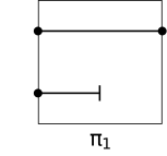
|
\begin {array}{lcl} \pi _0 : A \times B \rightarrow A & \qquad & \pi _1 : A \times B \rightarrow B \\ \pi _0(x, y) = x & & \pi _1(x, y) = y \\ \end {array} |
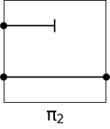
|
ConstructionProduct of cpos [dt-0021]
Given cpos A and B, the product A \times B is itself a cpo, ordered by (x,y) \sqsubseteq _{X \times Y} (x',y') \quad \text {iff} \quad x \sqsubseteq _X x' \land y \sqsubseteq _Y y' with bottom value \bot _{X \times Y} being (\bot _A, \bot _B). Least upper bounds are found by taking the lubs of each component:
\bigsqcup X \; = \; \left (\bigsqcup \{ \pi _0(x) \mid x \in X \}, \bigsqcup \{ \pi _1(x) \mid x \in X \}\right )TheoremContinuity of projection operations [dt-0022]
The projection functions \pi _0 and \pi _1 are continuous.
DefinitionThe split function [dt-0023]
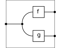
TheoremContinuity of split [dt-0024]
For continuous functions f and g, the split function \langle f, g \rangle is continuous.
Proof.
Using the alternative characterisation of continuity:
- \langle f, g \rangle is monotonic. Let x \sqsubseteq y \in A. Then: \begin {array}{lclr} \langle f , g \rangle \ x & = & (f(x), g(x)) & \text {(def)}\\ & \sqsubseteq & (f(y), g(y)) & \text {(monotonicity of $f$,$g$)}\\ & = & \langle f , g \rangle \ y & \text {(def)} \end {array}
- \langle f , g \rangle preserves lubs of directed sets. Let X \subseteq A be directed. Then: \begin {array}{lclr} \langle f , g \rangle \ (\bigsqcup X) & = & (f(\bigsqcup X), g(\bigsqcup X)) & \text {(def)}\\ & = & (\bigsqcup \{ f(x) \mid x \in X \}, \bigsqcup \{ g(x) \mid x \in X \}) & \text {(continuity of $f$,$g$)}\\ & = & \bigsqcup \{ \langle f , g \rangle \ x \mid x \in X \} & \text {(def)} \end {array}
These building blocks can be used to make many functions on products (thereby ensuring continuity):
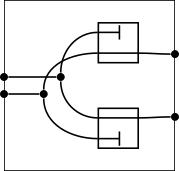
DefinitionThe \mathit {swap} function [dt-0025]
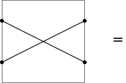 |
|
\begin {array}{l}\mathit {swap} : A \times B \rightarrow B \times A \\ \mathit {swap} = \langle \pi _1 , \pi _0 \rangle \end {array} |
DefinitionProduct of functions [dt-0026]
Given f : A \rightarrow C and g : B \rightarrow D, we overload the \times operator for products to denote the combined function f \times g : A \times B \rightarrow C \times D, given below:
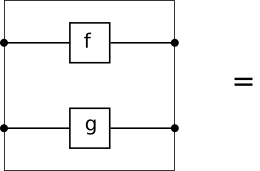 |
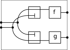 |
\begin {array}{l} f \times g : A \times B \rightarrow C \times D \\ f \times g = \langle f \circ \pi _0 , g \circ \pi _1 \rangle \end {array} |
Exercise [dt-002G]
Express the function \mathit {juggle} (a, (b,c)) = ((a,b),c) using just our primitive combinators for projection and split.
Solution.
\mathit {juggle} \triangleq \langle \langle \pi _0 , \pi _0 \circ \pi _1 \rangle , \pi _1 \circ \pi _1 \rangle
Pictorial Properties [dt-0027]
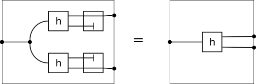
The following properties of our projection and split functions follow from the pictorial reasoning we see on the right:
| \pi _0 \circ \langle f , g \rangle = f | 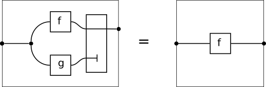 |
| \pi _1 \circ \langle f , g \rangle = g | 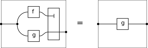 |
| \langle \pi _0 \circ h , \pi _1 \circ h \rangle = h |
 |
Exercise [dt-0028]
Prove that the three properties in § [dt-0027] are equivalent to the universal property for products
(\pi _0 \circ h = f \land \pi _1 \circ h = g)\ \text {iff}\ h = \langle f , g \rangleSolution.
Showing in both directions:
- The three properties follow from the universal property: The first two properties follow from the universal property where h is set to \langle f , g \rangle . The third property follows from the universal property where f is set to \pi _0\circ h and g is set to \pi _1\circ h.
- The universal property follows from the universal property: In the \Rightarrow direction of the universal property follows from the third property, and the \Leftarrow direction follows from the first two.
DefinitionUniversal property for cpo products [dt-0029]
As commuting diagram on the category \mathbf {Cpo}:
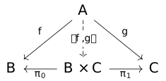
AsideCategory theory [dt-002A]
DefinitionCategory [dm-000G]
A category Cconsists of a collection of things (objects) and a collection of arrows between these things (morphisms). If there is a morphism A \xrightarrow {f} B and a morphism B \xrightarrow {g} C, we also have the composed morphism A \xrightarrow {g \circ f} C. This composition operator must be associative. Additionally each object X has an identity morphism X \xrightarrow {\mathsf {id}_X} X, such that for an arrow X \xrightarrow {a} Y, a \circ \mathsf {id}_X = \mathsf {id}_Y \circ a = a.
ExampleThe category \mathbf {Set} [dm-000H]
ExampleThe category \mathbf {Rel} [dm-000I]
ExampleThe category \mathbf {Cpo} [dt-002B]
The category \mathbf {Cpo} is the category where the objects are cpos, the morphisms are continuous functions between these cpos, composition is function composition ((g \circ f)(x) \triangleq g(f(x))) and identity is just the identity function \lambda x. x.
DefinitionFunctor [dm-000J]
A functor F from a category \mathbf {C} to a category \mathbf {D} consists of an object mapping that maps objects of \mathbf {C} to objects of \mathbf {D}, and a morphism mapping that maps morphisms of \mathbf {C} to morphisms of \mathbf {D} such that:
- For each A \xrightarrow {m} B in \mathbf {C}, we have a morphism F(A) \xrightarrow {F(m)} F(B) in \mathbf {D}.
- For each object A in \mathbf {C}, the equation F(\mathsf {id}_A) = \mathsf {id}_{F(A)} holds in \mathbf {D}.
- For a pair of morphism A \xrightarrow {f} B \xrightarrow {g} C in \mathbf {C}, the equation F (g \circ f) = F(g) \circ F(f) holds in \mathbf {D}.
ExampleThe category \mathbf {Cat} [dm-000K]
The category \mathbf {Cat} is the category where the objects are themselves (small) categories, the morphisms are structure-preserving maps between these categories, i.e., functors.
Commutative diagrams [dm-000L]
When working in a category, we can state many theorems compactly using commutative diagrams, such as this diagram for products:
CorollaryDerived properties of cpo products [dt-002C]
The universal property is called such because all the familiar properties of products follow from it – thinking in pictures helps to see how (Indeed, the universal property characterises products up to isomorphism):
- \pi _0 \circ (f \times g) = f \circ \pi _0
- \pi _1 \circ (f \times g) = g \circ \pi _1
- (f \times g) \circ \langle h , i \rangle = \langle f \circ h, g \circ i \rangle
- \langle f , g \rangle \circ h = \langle f \circ h, g \circ h \rangle
- \mathsf {id}_A \times \mathsf {id}_B = \mathsf {id}_{A \times B} \quad (*)
- (f \circ g) \times (h \circ i) = (f \times h) \circ (g \times i) \quad (**)
These last two statements (*) and (**) show that \times is a bifunctor on the category \textbf {Cpo}, i.e., a functor \textbf {Cpo} \times \textbf {Cpo} \rightarrow \textbf {Cpo}.
Exercise [dt-002I]
Show using the universal property that \langle f, g \rangle \circ h = \langle f \circ h , g \circ h \rangle
Solution.
Isomorphisms for cpo products [dt-002D]
DefinitionCpo isomorphism [dt-002E]
An isomorphism between two cpos A and B is a bijection f between A and B such that f preserves the cpo structure, i.e., that f and f^{-1} are continuous.
We say two cpos A and B are isomorphic, written A \simeq B, iff an isomorphism exists between them.
TheoremCommutative monoid structure for cpos [dt-002H]
Cpos form a commutative monoid "up to isomorphism" under \times and \mathbf {1} (the cpo consisting of only one element \bot ). That is, for all cpos A, B and C:
- A \times \mathbf {1} \simeq A
- A \times (B \times C) \simeq (A \times B) \times C
- A \times B \simeq B \times A
Proof.
The isomorphisms required are the projection \pi _0, the \mathit {juggle} function from Exercise [dt-002G], and the swap function.
DefinitionThe set of continuous functions [dt-002F]
Let A \twoheadrightarrow B denote just the continuous functions from cpo A to cpo B: A \twoheadrightarrow B\; \triangleq \; \{ f : A \rightarrow B \mid f\ \text {is continuous} \}
Theorem [dt-002J]
There is an isomorphism between pairs of continuous functions and continuous functions that output pairs: (A \twoheadrightarrow B) \times (A \twoheadrightarrow C)\; \simeq \; (A \twoheadrightarrow (B \times C))
Proof.
Upshot.
Because we have the functor \times on \textbf {Cpo} that satisfies the properties of products described above, the category \textbf {Cpo} therefore has binary products.
Functions [dt-002Z]
Previously, such as in Example [dt-001U], we already implicitly assumed that the set of continuous functions on cpos A \twoheadrightarrow B is itself a cpo. In this section, we will formalise this construction.
ConstructionThe cpo of functions [dt-002L]
If A and B are cpos, the set of continuous functions A \twoheadrightarrow B is a cpo under the pointwise ordering: f \sqsubseteq g\;\; \text {iff}\;\; \forall a \in A.\ f(a) \sqsubseteq g(a) The intuition of this ordering in terms of information is that we increase the information content of a function overall by increasing the information content of any (or many) argument values. To prove this, we must show:
- A \twoheadrightarrow B has a least element. \bot _{A \twoheadrightarrow B} is the constant function that returns \bot _B, i.e. \lambda a.\ \bot _B.
- \bigsqcup X exists for all directed X \subseteq A \twoheadrightarrow B. Our lub of a set of continuous functions \bigsqcup X is the function \Phi where: \Phi (a) = \bigsqcup \{ f(a) \mid f \in X\}
We must show a number of properties of this lub \Phi . Specifically:
- \bigsqcup \{ f(a) \mid f \in X\} exists in B.
Proof.
We want to show that the set \{ f(a) \mid f \in X\} is directed. Take two values g(a), h(a) \in \{ f(a) \mid f \in X\}. Since X is directed, there exists a function k \in X such that g \sqsubseteq k and h \sqsubseteq k. By applying the definition of \sqsubseteq for functions above, we have g(a) \sqsubseteq k(a) and h(a) \sqsubseteq k(a). Thus k(a) is an upper bound of these two values g(a), h(a), and thus \{ f(a) \mid f \in X\} is directed, and thus its lub exists since B is a cpo. - \Phi (a) = \bigsqcup \{ f(a) \mid f \in X \} is continuous.
Proof.
Using the alternative characterisation of continuity
\begin {array}{lclr} \Phi (\bigsqcup Y) &=& \bigsqcup \{ f(\bigsqcup Y) \mid f \in X \} & \text {(defn. $\Phi $)}\\ & = & \bigsqcup \{\bigsqcup \{ f(y) \mid y \in Y \} \mid f \in X \} & \text {($f$ is continuous)}\\ & = & \bigsqcup \{\bigsqcup \{ f(y) \mid f \in X \} \mid y \in Y \} & \text {(swap lubs)}\\ & = & \bigsqcup \{ \Phi (y) \mid y \in Y \} & \text {(defn. $\Phi $)}\\ \end {array} Monotonicity is similar to prove. - \Phi is an upper bound for X \subseteq A \twoheadrightarrow B.
Proof.
Let g \in X. Then for any a \in A we have g(a) \in \{ f(a) \mid f \in X\}. Now, by 2a and lubs, we have g(a) \sqsubseteq \bigsqcup \{ f(a) \mid f \in X \}, which by the definition of \Phi gives g(a) \sqsubseteq \Phi (a). Hence, by the definition of \sqsubseteq on functions, we can conclude g \sqsubseteq \Phi . - \Phi is the least upper bound for X.
Proof.
Let g \in A \twoheadrightarrow B be an upper bound for X \subseteq A \twoheadrightarrow B. Then (using \sqsubseteq on functions) g(a) is an upper bound for \{f(a) \mid f \in X\} for all a \in A. Now, by 2a and lubs, we have \bigsqcup \{f(a) \mid f \in X\} \sqsubseteq g(a), i.e. \Phi (a) \sqsubseteq g(a), which, by the definition of \sqsubseteq on functions, allows us to conclude \Phi \sqsubseteq g.
- \bigsqcup \{ f(a) \mid f \in X\} exists in B.
ExampleThe space \mathbb {B}_\bot \twoheadrightarrow \mathbb {B}_\bot [dt-002M]
 At each step "upwards" on this
Primitive functions for functions [dt-002P]
DefinitionThe \mathit {apply} function [dt-002N]
The \mathit {apply} function simply applies a given function to a given argument: \begin {array}{l} \mathit {apply} : ((A \twoheadrightarrow B) \times A) \twoheadrightarrow B\\ \mathit {apply} (f, a) = f(a) \end {array}
Exercise [dt-002Q]
Show that \mathit {apply} is continuous.
Hint: A function f : A \times B \rightarrow C is continuous iff it is continuous in each argument separately, i.e., iff \forall a \in A.\ f(a,\cdot ) : B \rightarrow C is continuous, and \forall b \in B.\ f(\cdot ,b) : A \rightarrow C is continuous.
Solution.
First showing \mathit {apply}(f,\cdot ) is continuous for some continuous f : A \twoheadrightarrow B, using the alternative characterisation
- \mathit {apply}(f,\cdot ) is monotonic: Given a, b \in A where a \sqsubseteq b, we can see that \mathit {apply}(f,a) = f(a) \sqsubseteq f(b) = \mathit {apply}(f,b) by the monotonicity of f.
- \mathit {apply}(f,\cdot ) preserves lubs: Given a directed X \subseteq A, we can see that \mathit {apply}(f,\bigsqcup X) = f(\bigsqcup X) = \bigsqcup \{f(x) \mid x \in X\} = \bigsqcup \{\mathit {apply}(f,x) \mid x \in X\} follows from the continuity of f.
- \mathit {apply}(\cdot ,a) is monotonic: Given f, g \in A \twoheadrightarrow B where f \sqsubseteq g, we can see that \mathit {apply}(f,a) = f(a) \sqsubseteq g(a) = \mathit {apply}(g,a) by the pointwise ordering of functions.
- \mathit {apply}(\cdot ,a) preserves lubs: Given a directed X \subseteq A \twoheadrightarrow B, we can see that \mathit {apply}(\bigsqcup X, a) = \left (\bigsqcup X\right )(a) = \bigsqcup \{f(a) \mid f \in X\} = \bigsqcup \{\mathit {apply}(f,a) \mid f \in X\} follows from the lub definition for functions.
DefinitionThe \mathit {curry} function [dt-002O]
The function \mathit {curry} transforms a function that takes two arguments all at once (as a product) into a function that takes the arguments one at a time. That is, if f : A \times B \twoheadrightarrow C then: \begin {array}{l} \mathit {curry}(f) : A \twoheadrightarrow (B \twoheadrightarrow C)\\ \mathit {curry}(f)(a)(b) = f(a, b) \end {array}
TheoremContinuity of \mathit {curry} [dt-002S]
- \mathit {curry} is continuous on A \times B \twoheadrightarrow C.
- \mathit {curry}(f), given continuous f : A \times B \twoheadrightarrow C, is continuous on A.
- \mathit {curry}(f)(a), given continuous f : A \times B \twoheadrightarrow C and a \in A, is continuous on B.
Exercise [dt-002R]
What is the common (functional programming) name for \mathit {apply} \circ (f \times \mathsf {id})?
\mathit {uncurry}Solution.
DefinitionUniversal property for functions [dt-002T]
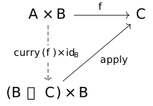
TheoremThe currying isomorphism [dt-002U]
Proof.
Follows from the universal property for functions when set up with the isomorphism from curry and its inverse, the function in Exercise [dt-002R].
RemarkWhy the function arrow is not a covariant bifunctor [dt-002V]
For the \twoheadrightarrow operator on cpos (Definition [dt-002F]) to be the object mapping for a bifunctor \textbf {Cpo} \times \textbf {Cpo} \rightarrow \textbf {Cpo} like \times is (see Corollary [dt-002C]), we would need to define a morphism mapping f \twoheadrightarrow g that, given two functions f : A \twoheadrightarrow B and g : C \twoheadrightarrow D, gives a function (A \twoheadrightarrow C) \twoheadrightarrow (B \twoheadrightarrow D). But such a function is not implementable: \begin {array}{l} f \twoheadrightarrow g : (A \twoheadrightarrow C) \twoheadrightarrow (B \twoheadrightarrow D) \\ (f \twoheadrightarrow g)(h)(b) =\ \textcolor {red}{???}\\ \end {array} In the above hole \textcolor {red}{???}, h : A \twoheadrightarrow C and b \in B. Given the value b \in B, none of our functions f, g or h take elements of B, so there would be no way to produce the D value required. This is because our function f : A \twoheadrightarrow B goes the wrong way. If f were a function B \twoheadrightarrow A, things would be a lot easier.
DefinitionDual category [dm-000Q]
The function arrow is a bifunctor [dt-002W]
The operator \twoheadrightarrow introduced in Definition [dt-002F] is is the object mapping for a binary functor: (\twoheadrightarrow ) : \mathbf {Cpo}^\mathsf {op} \times \mathbf {Cpo} \rightarrow \mathbf {Cpo} The category \mathbf {Cpo}^\mathsf {op} is the dual category to \mathbf {Cpo}.
Thus, a morphism A \xrightarrow {m} B in the category \mathbf {Cpo}^\mathsf {op} is a continuous function m : B \twoheadrightarrow A. Thus, the morphism mapping for our functor must take two functions f : B \twoheadrightarrow A (the morphism from \mathbf {Cpo}^\mathsf {op}) and g : C \twoheadrightarrow D (the morphism from \mathbf {Cpo}), and produce (A \twoheadrightarrow C) \twoheadrightarrow (B \twoheadrightarrow D). As with products, we will overload the \twoheadrightarrow notation for this mapping as well.
DefinitionMorphism mapping for \twoheadrightarrow [dt-002X]
Given f : B \twoheadrightarrow A and g : C \twoheadrightarrow D, we have: \begin {array}{l} f \twoheadrightarrow g : (A \twoheadrightarrow C) \twoheadrightarrow (B \twoheadrightarrow D)\\ f \twoheadrightarrow g = \mathit {curry}\ (g \circ \mathit {apply} \circ (\mathsf {id} \times f))\\[2em] \text {(or, operationally:)}\\ (f \twoheadrightarrow g)(h) = g \circ h \circ f\\ \end {array}
Theorem [dt-002Y]
The two functor laws follow as a consequence of the universal property for functions:
- \mathsf {id}_A \twoheadrightarrow \mathsf {id}_B = \mathsf {id}_{A \twoheadrightarrow B}
- (f \circ g) \twoheadrightarrow (h \circ i) = (g \twoheadrightarrow h) \circ (f \twoheadrightarrow i)
Upshot.
Our category \textbf {Cpo} has exponentials.
Sums [dt-0030]
ConstructionSum of cpos [dt-0031]
The sum construct on cpo A + B denotes a disjoint union of two cpos with a new, dedicated \bot value: A + B = \{ (0, a) \mid a \in A \} \cup \{ (1, b) \mid b \in B \} \cup \{ \bot _{A+B} \} This construct is a cpo under the ordering: x \sqsubseteq y\;\;\text {iff}\;\;\begin {cases} \text {true} & \text {if}\ x=\bot _{A+B}\\ a \sqsubseteq a' & \text {if}\ x = (0,a)\ \text {and}\ y = (0, a') \\ b \sqsubseteq b' & \text {if}\ x = (1,b)\ \text {and}\ y = (1, b') \\ \text {false} & \text {otherwise} \end {cases} Intuitively, this says that the ordering on A + B is the same as A and B separately, except that \bot _{A+B} is less than anything.
The only directed sets are those that do not contain a mixture of elements from both A and from B, so the least upper bound operator is essentially the same as the least upper bounds for A and for B. Formally: \bigsqcup X \;\; = \;\; \begin {cases} (0,\bigsqcup \{ a \mid (0,a) \in X \}) & \text {if}\ \{ a \mid (0,a) \in X \} \neq \emptyset \\ (1,\bigsqcup \{ b \mid (1,b) \in X \}) & \text {if}\ \{ b \mid (1,b) \in X \} \neq \emptyset \\ \bot _{A+B} & \text {otherwise}\\ \end {cases}
Primitive functions for sums [dt-003D]
DefinitionConstructors for sums [dt-0032]
For constructing sums, we use two primitive constructor functions, \mathit {inl} and \mathit {inr}: \begin {array}{l} \mathit {inl} : A \twoheadrightarrow (A + B)\\ \mathit {inl}(x) = (0,x)\\[1em] \mathit {inr} : B \twoheadrightarrow (A + B)\\ \mathit {inr}(y) = (1,y) \end {array}
TheoremContinuity of sum constructors [dt-0033]
The constructor functions \mathit {inl} and \mathit {inr} are continuous.
DefinitionThe case function [dt-0034]
Elimination of sums is captured by the case function [f,g] : (A + B) \twoheadrightarrow C, made from functions f : A \twoheadrightarrow C and g : B \twoheadrightarrow C. This function is defined by: \begin {array}{l} [f,g] : (A + B) \twoheadrightarrow C\\ [f,g](x) = \begin {cases} f(a) & \text {if}\ x = (0,a) \\ g(b) & \text {if}\ x = (1,b) \\ \bot _C & \text {if}\ x = \bot _{A+B}\end {cases} \end {array}
Exercise [dt-0035]
Prove that the case function [f,g](x) is, given continuous functions f : A \twoheadrightarrow C and g : B \twoheadrightarrow C, continuous on its argument x.
As mentioned in Construction [dt-0031], the only directed subsets of A + B are those that contain entirely values of the format (0,\_) and optionally \bot _{A+B}, or those that contain entirely values of the format (1,\_) and optionally \bot _{A+B}. Call this directed subset X.
Solution.
Locality of sums [dt-0039]
We can see by the definitions of case and our constructors that [f,g] \circ \mathit {inl} = f and [f,g] \circ \mathit {inr} = g, or, in a commutative diagram:
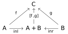
Note that this diagram is like the dual of the diagram seen in the universal property for products — the arrows are reversed. That is because, generally speaking, sums are dual to products. However, because of our additional \bot value, our cpo sums are only weakly universal — the h arrow is not unique.
ExampleWeak universality of cpo sums [dt-003A]
Consider this scenario with the cpos \textbf {2} = \{ \top , \bot \} and \textbf {1} = \{\bot \}:
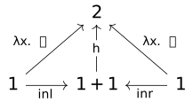
DefinitionWeak universal property for cpo sums [dt-003B]
This property is called weak because it uses only the information ordering rather than equality on the right hand side.
WarningFailure of sum isomorphisms [dt-003C]
The weakness of the universal property for sums means that many common isomorphisms for sums in other contexts do not hold:
- A + (B + C) \not \simeq (A + B) + C
- (A \twoheadrightarrow C) \times (B \twoheadrightarrow C) \not \simeq (A+B) \twoheadrightarrow C
Sums form a bifunctor [dt-0036]
With these, we can define the morphism mapping for the sum bifunctor (+) : \textbf {Cpo} \times \textbf {Cpo} \rightarrow \textbf {Cpo}. Just as with products and functions, we will overload the + notation for morphisms as well as objects in the category \mathbf {Cpo}.
DefinitionSum of functions [dt-0037]
Given functions f : A \twoheadrightarrow C and g : B \twoheadrightarrow D, we have: \begin {array}{l} f+g : (A + B)\twoheadrightarrow (C + D) \\ f+g = [\mathit {inl} \circ f, \mathit {inr} \circ g] \end {array}
Theorem [dt-0038]
+ : \mathbf {Cpo} \times \mathbf {Cpo} \rightarrow \mathbf {Cpo} is a lawful bifunctor, that is:
- (\lambda a. a) \times (\lambda b. b) = (\lambda x.x)
- (f_1 \circ g_1) \times (f_2 \circ g_2) = (f_1 \times f_2) \circ (g_1 \times g_2)
Upshot.
Our category \mathbf {Cpo} has only local sums.
Strict Constructions [dt-003E]
When giving a semantics to a call-by-name (or "lazy") language, the constructions \twoheadrightarrow for functions, \times for products and + for sums are exactly what we want. To properly capture call-by-value (or "strict") languages, however, we also need strict versions of these constructions.
ConstructionThe cpo of strict continuous functions [dt-003F]
The ordering and lubs are, mutatis mutandis, as with the non-strict Construction [dt-002L].
ConstructionSmash products of cpos [dt-003G]
The ordering and lubs are, mutatis mutandis, as with the non-strict Construction [dt-0021]. This operator is called a smash product because the two \bot values from A and B are "smashed" into one \bot value.
ConstructionSmash sums of cpos [dt-003H]
The ordering and lubs are, mutatis mutandis, as with the non-strict Construction [dt-0031]. This operator is called a smash sum because the two \bot values from A and B are "smashed" into one \bot value.
TheoremIsomorphisms with strict constructions [dt-003J]
The strict cpo constructions satisfy all the usual isomorphisms, including:
- (A \mathbin {\circ \hspace{-0.4em}\twoheadrightarrow } B) \times (A \mathbin {\circ \hspace{-0.4em}\twoheadrightarrow } C)\;\; \simeq \;\; A \mathbin {\circ \hspace{-0.4em}\twoheadrightarrow } (B\otimes C)
- (A \otimes B \mathbin {\circ \hspace{-0.4em}\twoheadrightarrow } C) \;\; \simeq \;\; A \mathbin {\circ \hspace{-0.4em}\twoheadrightarrow } (B \mathbin {\circ \hspace{-0.4em}\twoheadrightarrow } C)
- (A \mathbin {\circ \hspace{-0.4em}\twoheadrightarrow } C) \times (B \mathbin {\circ \hspace{-0.4em}\twoheadrightarrow } C)\;\; \simeq \;\; (A\oplus B) \mathbin {\circ \hspace{-0.4em}\twoheadrightarrow } C
DefinitionThe category \mathbf {Cpo_\bot } [dt-003I]
The category \mathbf {Cpo_\bot } is the category where the objects are cpos, the morphisms are strict continuous functions between these cpos, and composition and identity are as in \mathbf {Cpo}.
Upshot.
DefinitionThe lifting operator for cpos [dt-003K]
TheoremIsomorphisms with lifting [dt-003L]
With the lifting operator, we can relate the lazy constructions like product and sum with strict constructions like smash product and sum via isomorphism:
- A\twoheadrightarrow B \simeq A_\bot \mathbin {\circ \hspace{-0.4em}\twoheadrightarrow } B
- A + B \simeq A_\bot \oplus B_\bot
- (A \times B)_\bot \simeq A_\bot \otimes B_\bot
PCF [dt-003T]
For most purposes in semantics, describing semantics in terms of (continuous functions on) cpos is enough. To demonstrate, we will give semantics to PCF: a Turing-complete, higher order functional programming language. We will then extend PCF to include more features, namely pairs (product types) and sum types.
DefinitionThe language PCF [dt-003M]
The language for Programming Computable Functions (PCF) is a variant of typed \lambda -calculus with minimal extensions to be Turing-complete. \begin {array}{lcl} e & \Coloneqq & n \mid x \mid \lambda x : \tau .\ e \mid e_1\ e_2\mid \mathsf {succ} \mid \mathsf {pred} \mid \mathsf {ifz}\ e_1\ \mathsf {then}\ e_2\ \mathsf {else}\ e_3 \mid \mathsf {fix}\ x : \tau .\ e \\ \tau & \Coloneqq & \mathsf {nat} \mid \tau _1 \rightarrow \tau _2 \end {array}
DefinitionTyping rules for PCF [dt-003N]
\dfrac {n \in \mathbb {N}}{\Gamma \vdash n : \mathsf {nat}}\quad \dfrac {x : \tau \in \Gamma }{\Gamma \vdash x : \tau }\quad \dfrac {\Gamma , x : \tau _1 \vdash e : \tau _2 }{ \Gamma \vdash \lambda x : \tau _1.\ e : \tau _1 \rightarrow \tau _2}\quad \dfrac {\Gamma \vdash e_1 : \tau _1 \rightarrow \tau _2 \quad \Gamma \vdash e_2 : \tau _1}{\Gamma \vdash e_1\ e_2 : \tau _2}\\[2em] \dfrac { }{ \Gamma \vdash \mathsf {succ} : \mathsf {nat} \rightarrow \mathsf {nat}}\quad \dfrac { }{ \Gamma \vdash \mathsf {pred} : \mathsf {nat} \rightarrow \mathsf {nat}}\quad \dfrac { \Gamma \vdash e_1 : \mathsf {nat} \quad \Gamma \vdash e_2 : \tau \quad \Gamma \vdash e_3 : \tau }{ \Gamma \vdash \mathsf {ifz}\ e_1\ \mathsf {then}\ e_2\ \mathsf {else}\ e_3 : \tau }\quad \dfrac { \Gamma , x : \tau \vdash e : \tau }{\Gamma \vdash \mathsf {fix}\ x : \tau .\ e : \tau }
Type-dependent denotations [dt-003O]
Because PCF is typed, we shall assign denotations only to well-typed expressions. The range of our denotation function for expressions is determined by the type of its input expression. That is, the denotation of a type \tau is the cpo whose elements will be the denotations of expressions of type \tau . The denotation of the type \mathsf {nat}, then, is merely the flat domain of the natural numbers \mathbb {N}_\bot : \llbracket \mathsf {nat} \rrbracket = \mathbb {N}_\bot And, the denotation of the function type is the domain of continuous functions on cpos: \llbracket \tau _1 \rightarrow \tau _2 \rrbracket = \llbracket \tau _1 \rrbracket \twoheadrightarrow \llbracket \tau _2 \rrbracket A closed term e : \tau with no free variables denotes an element of \llbracket \tau \rrbracket , so we might be tempted to define our denotation function for expressions e : \tau like so: \llbracket e \rrbracket : \llbracket \tau \rrbracket However, if e : \tau involves free variables from our context \Gamma , the valuation of e will depend on the values assigned to all the variables. Thus, the denotation of a typed expression \Gamma \vdash e : \tau is defined instead as a continuous function: \llbracket e \rrbracket _\Gamma : \llbracket \Gamma \rrbracket \twoheadrightarrow \llbracket \tau \rrbracket where the meaning of a context \Gamma = (x_0 : \tau _0, x_1 : \tau _1,\dots , x_n : \tau _n) will be a a big n-tuple of the values assigned to each variable: \llbracket \Gamma \rrbracket = \llbracket \tau _0 \rrbracket \times \llbracket \tau _1 \rrbracket \times \cdots \times \llbracket \tau _n \rrbracket
DefinitionNotation for n-tuples [dt-003Q]
Given an n-tuple, i.e. elements of the n-ary product X_0 \times X_1 \times X_2 \times \dots \times X_n, we typically denote the entire n-tuple as in vector notation: \vec {x} : X_0 \times X_1 \times X_2 \times \dots \times X_n And individual elements of the tuple are accessed with numeric subscripts: x_0 : X_0 \quad x_2 : X_2 \quad \cdots
DefinitionSemantics of PCF [dt-003P]
Types
Expressions
Extending PCF with product types [dt-003R]
We shall extend the syntax of PCF with a new type former, \tau _1 \times \tau _2 and three expression-level constructs for constructing and deconstructing pairs: \begin {array}{lcl} e & \Coloneqq & \cdots \mid (e_1,e_2) \mid \mathsf {fst}\ e \mid \mathsf {snd}\ e \\ \tau & \Coloneqq & \cdots \mid \tau _1 \times \tau _2 \end {array} Adding to our typing rules similarly: \dfrac {\Gamma \vdash e_1 : \tau _1 \quad e_2 : \tau _2}{(e_1,e_2) : \tau _1 \times \tau _2}\\[2em] \dfrac {\Gamma \vdash e : \tau _1 \times \tau _2}{\Gamma \vdash \mathsf {fst}\ e : \tau _1}\quad \dfrac {\Gamma \vdash e : \tau _1 \times \tau _2}{\Gamma \vdash \mathsf {snd}\ e : \tau _2} To extend our semantics, we make the product type \tau _1 \times \tau _2 denote the product cpo \llbracket \tau _1 \rrbracket \times \llbracket \tau _2 \rrbracket , and our expression semantics are expressed straightforwardly using our projection and split operations for products: \begin {array}{lcl} \llbracket (e_1, e_2) \rrbracket _\Gamma &=& \langle \llbracket e_1 \rrbracket _\Gamma , \llbracket e_2 \rrbracket _\Gamma \rangle \\ \llbracket \mathsf {fst}\ e \rrbracket _\Gamma & = & \pi _0 \circ \llbracket e \rrbracket _\Gamma \\ \llbracket \mathsf {snd}\ e \rrbracket _\Gamma & = & \pi _1 \circ \llbracket e \rrbracket _\Gamma \\ \end {array}
Extending PCF with sum types [dt-003S]
We shall extend the syntax of PCF with a new type former, \tau _1 + \tau _2 and three expression-level constructs for constructing and deconstructing sums: \begin {array}{lcl} e & \Coloneqq & \cdots \mid \mathsf {inl}\ e \mid \mathsf {inr}\ e \mid \mathsf {case}\ e_0\ \mathsf {of}\ \mathsf {inl}\ x \rightarrow e_1 ; \mathsf {inr}\ y \rightarrow e_2 \\ \tau & \Coloneqq & \cdots \mid \tau _1 + \tau _2 \end {array} Adding to our typing rules similarly: \dfrac {\Gamma \vdash e : \tau _1}{\Gamma \vdash \mathsf {inl}\ e : \tau _1 + \tau _2}\quad \dfrac {\Gamma \vdash e : \tau _2}{\Gamma \vdash \mathsf {inr}\ e : \tau _1 + \tau _2}\\[2em] \dfrac {\Gamma \vdash e_0 : \tau _1 + \tau _2 \quad \Gamma , x : \tau _1 \vdash e_1 : \tau \quad \Gamma , y : \tau _2 \vdash e_2 : \tau }{ \Gamma \vdash \mathsf {case}\ e_0\ \mathsf {of}\ \mathsf {inl}\ x \rightarrow e_1 ; \mathsf {inr}\ y \rightarrow e_2 : \tau } To extend our semantics, we make the sum type \tau _1 + \tau _2 denote the sum cpo \llbracket \tau _1 \rrbracket + \llbracket \tau _2 \rrbracket , and our expression semantics are expressed using our primitive functions for sums. \begin {array}{lcl} \llbracket \mathsf {inl}\ e \rrbracket _\Gamma & = & \mathit {inl} \circ \llbracket e \rrbracket _\Gamma \\ \llbracket \mathsf {inr}\ e \rrbracket _\Gamma & = & \mathit {inr} \circ \llbracket e \rrbracket _\Gamma \end {array} \begin {array}{l}\llbracket \mathsf {case}\ e_0\ \mathsf {of}\ \mathsf {inl}\ x \rightarrow e_1 ; \mathsf {inr}\ y \rightarrow e_2 \rrbracket _\Gamma (\vec {z}) \\ \quad = [ \boldsymbol {\lambda }v. \llbracket e_1 \rrbracket _{\Gamma ,x:\tau _1}(\vec {z},v), \boldsymbol {\lambda }v. \llbracket e_2 \rrbracket _{\Gamma ,y:\tau _2}(\vec {z},v)] (\llbracket e_0 \rrbracket _\Gamma (\vec {z}))\end {array}
LectureRecursively defined domains and \lambda -calculus [dt-004Z]
This lecture is based on material from Graham Hutton, John Longley, Dana Scott, Joseph Stoy, Carl Gunter, and Glynn Winskel.
Why we need recursively defined domains [dt-004J]
We saw recursive domain equations with higher-order procedures in § [dt-0007], but there are numerous other examples where they come up.
Recursive algebraic data types [dt-004L]
Suppose we have a language with recursive data types, such as this \mathit {List} type in Haskell-style syntax: \textbf {data}\ \mathit {List} = \mathsf {Nil} \mid \mathsf {Cons}\ (\mathit {Int} \times \mathit {List}) As in PCF, the denotation of a type \tau is the domain which contains all the denotations of all closed expressions of type \tau . What, then, is the domain that corresponds to \mathit {List}\ a? We need a cpo L that satisfies the below equation (where \mathbf {1} is the cpo containing just one element \bot ): L \simeq \mathbf {1} + (\mathbb {Z}_\bot \times L)
Untyped higher-order languages [dt-004M]
If we take PCF, discard the type system, \textbf {fix}, natural number primitives and any other superfluous features, and just boil our language down to a minimal, Turing-complete subset, we end up with the untyped \lambda -calculus — a language consisting only of untyped functions.
DefinitionUntyped \lambda -calculus [dt-004K]
Untyped \lambda -calculus consists only of untyped (higher-order) functions: e \; \Coloneqq \; x \mid \lambda x. e \mid e_1\ e_2
Trying to give a semantics to the untyped \lambda calculus poses an issue: we can no longer rely on the type of an expression to select an appropriate semantic domain. Instead, we we must pick a single domain D which, since functions can be applied to themselves, must apparently include the set of functions D \twoheadrightarrow D: D \simeq D\twoheadrightarrow D
How can we find solutions to such recursive equations? How can we guarantee the existence of a (least) solution?
We can start by generalising the fixed point approach we used for values (i.e. elements of cpos) to domains (i.e. cpos themselves).
ExampleRecursive domain equations as endofunctors [dt-004N]
This recursive equation for lists: L \simeq \mathbf {1} + (\mathbb {Z}_\bot \times L) Can be expressed as the least fixed point of this mapping (specifically an endofunctor) \mathcal {F} on cpos: \mathcal {F}(A) \triangleq \mathbf {1} + (\mathbb {Z}_\bot \times A)
To ensure that least fixed points exist, and to give us a means of finding them, we must now generalise all of the concepts we used for least fixed points on values (information ordering, least upper bounds, continuity etc.) to domains themselves.
From a cpo to the category \mathbf {Cpo} [dt-004O]
Problem.
The following definitions are insufficient when using function constructions in our domain equations (\twoheadrightarrow and \mathbin {\circ \hspace{-0.4em}\twoheadrightarrow }), but it will suffice for our purposes for now.
Let us say (for now) that a cpo A approximates a cpo B (i.e. A \sqsubseteq B) iff there is a continuous function f : A\twoheadrightarrow B. Then, there is a least element for this ordering: the one-element cpo \mathbf {1} = \{ \bot \}, as the continuous function (\lambda x. \bot ) : \mathbf {1} \twoheadrightarrow A exists for any cpo A.
Categorical Aside. Initiality
The category \mathbf {Cpo} has no initial object. The cpo \mathbf {1} is terminal; but also serves as a "pseudo" initial object due to the above.
Colimits in the category \mathbf {Cpo} [dt-004P]
Definition\omega -chains of cpos in the category \mathbf {Cpo} [dt-004Q]
An \omega -chain of cpos in the category \mathbf {Cpo} consists of a family of cpos \{A_i \mid i \in \mathbb {N} \}, together with a family of continuous functions \{ f_i : A_i\twoheadrightarrow A_{i+1} \mid i \in \mathbb {N}\}, shown below:

DefinitionUpper bounds in the category \mathbf {Cpo} [dt-004R]
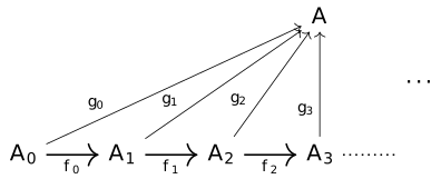
A cpo A is an upper bound of an \omega -chain of cpos in the category \mathbf {Cpo} if there is a family of continuous functions \{g_i : A_i \twoheadrightarrow A \mid i \in \mathbb {N}\} such that the following diagram commutes (i.e. g_i = g_{i+1} \circ f_i for all i \in \mathbb {N}):
DefinitionLeast upper bounds in the category \mathbf {Cpo} [dt-004S]
A cpo A is the least upper bound of an \omega -chain of cpos if is both an upper bound and if there exists a unique k for any other upper bound B such that the following diagram commutes (i.e. h_i = k \circ g_i for all i \in \mathbb {N}):
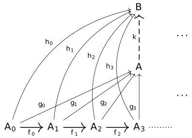
The least upper bound of such an \omega -chain is also called its colimit.
Note: Uniqueness of lubs is up to isomorphism. That is, if A and B are both colimits of our \omega -chain, then A \simeq B.
DefinitionEndofunctors on \textbf {Cpo} [dt-004T]
An endofunctor on the category \textbf {Cpo} is a functor \textbf {Cpo} \rightarrow \textbf {Cpo}, i.e. a mapping \mathcal {F} on cpos together with a mapping \mathcal {F} on continuous functions, such that:
- If f : A \twoheadrightarrow B then \mathcal {F}(f) : \mathcal {F}(A)\twoheadrightarrow \mathcal {F}(B)
- \mathcal {F}(\mathsf {id}_A : A\twoheadrightarrow A) = \mathsf {id}_{\mathcal {F}(A)} : \mathcal {F}(A)\twoheadrightarrow \mathcal {F}(A)
- \mathcal {F}(f \circ g) = \mathcal {F}(f) \circ \mathcal {F}(g)
Remark [dt-004U]
Observe that, given the information ordering for cpos where A \sqsubseteq B if there exists a continuous function A \twoheadrightarrow B, the functor laws necessarily imply monotonicity for all endofunctors \mathcal {F}.
DefinitionCocontinuous endofunctors [dt-004V]
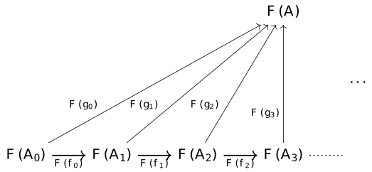
An endofunctor \mathcal {F} is cocontinuous iff it preserves colimits of \omega -chains of cpos. That is, given a chain where A is a colimit:
DefinitionFixed points of endofunctors on \mathbf {Cpo} [dt-004W]
A fixed point of an endofunctor on cpos \mathcal {F} is a cpo \mathcal {F} such that \mathcal {F}(A) \simeq A.
Note.
In Scott's approach, which we follow here, our fixed points are up to isomorphism (suitable for languages with isorecursive types), but there are other approaches where they are equalities (suitable for languages with equirecursive types).
TheoremFixed point theorem for endofunctors on \mathbf {Cpo} [dt-004X]
Every cocontinuous endofunctor \mathcal {F} on cpos has a least fixed point, given by the colimit of the \omega -chain:

ExampleBinary Numbers [dt-004Y]
Consider the Haskell-style data type: \textbf {data}\ \mathit {Bin} = \mathsf {Zero}\ \mathit {Bin} \mid \mathsf {Empty} \mid \mathsf {One}\ \mathit {Bin} So, e.g. \mathsf {One}\ (\mathsf {Zero}\ (\mathsf {One}\ \mathsf {Empty})) : \mathit {Bin}.
The recursive domain equation is, expressed as a fixed point: B \simeq \mathcal {F}(B)\quad \text {where}\ \mathcal {F}(X) = X + \mathbf {1} + X We wish to show that \mathcal {F} is a cocontinuous endofunctor.
We have a mapping \mathcal {F} on cpos (objects of the category \textbf {Cpo}), but for it to be a functor we additionally need a mapping \mathcal {F} on continuous functions (morphisms of the category \textbf {Cpo}).
Recalling our sum construction, we may remember that sums are already a bifunctor \textbf {Cpo} \times \textbf {Cpo} \rightarrow \textbf {Cpo} (Theorem [dt-0038]). Thus, our mapping on continuous functions \mathcal {F} can be derived from our mapping on cpos \mathcal {F} by using the morphism mapping from the sum construction (Definition [dt-0037]). Given a continuous function f : A \twoheadrightarrow B, our morphism mapping is:
\begin {array}{l} \mathcal {F}(f) : \mathcal {F}(A)\twoheadrightarrow \mathcal {F}(B)\\ \mathcal {F}(f) \triangleq f + \mathsf {id}_\textbf {1} + f \end {array}Proof that this endofunctor is cocontinuous is left for the reader. Hence the semantics of the type \mathit {Bin}, i.e. \llbracket \mathit {Bin} \rrbracket : \textbf {Cpo} is the least fixed point of \mathcal {F}, i.e. the colimit of the \omega -chain:

Let us visualise this chain. Here the sum injections have been written as \textsf {Z, E, O} rather than (combinations of) \textsf {inl} and \textsf {inr} to keep the connection with the Haskell data type clear.
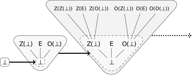
Thus, the nth cpo in the chain contains binary numbers with at most n defined digits. The colimit of the chain contains all binary numbers (finite, partial, and infinite!).
Exercise [dt-005M]
Show that \mathcal {F}(X) \triangleq \mathbf {1} + X and \mathcal {F}(f) \triangleq \mathsf {id}_\mathbf {1} + f (using our + operator for functions) define an endofunctor \mathbf {Cpo} \rightarrow \mathbf {Cpo}, i.e. that they satisfy the functor laws.
Solution.
- We must show \mathcal {F}(\mathsf {id}_A : A \twoheadrightarrow A) = \mathsf {id}_{\mathcal {F}(A)} : \mathcal {F}(A) \twoheadrightarrow \mathcal {F}(A). \begin {array}{lcl} \mathcal {F}(\mathsf {id}_A)& =& \mathsf {id}_\mathbf {1} + \mathsf {id}_A\\ &=& \mathsf {id}_{\mathbf {1} + A}\\ &=& \mathsf {id}_{\mathcal {F}(A)} \end {array}
- We must show \mathcal {F}(f \circ g) = \mathcal {F}(f) \circ \mathcal {F}(g). \begin {array}{lcl} \mathcal {F}(f \circ g) &=& \mathsf {id}_\mathbf {1} + (f \circ g) \\ &=& (\mathsf {id}_\mathbf {1} + f) \circ (\mathsf {id}_\mathbf {1} + g) \\ & = & \mathcal {F}(f) \circ \mathcal {F}(g) \end {array}
Constructing endofunctors [dt-0050]
If we have a mapping on cpos \mathcal {F} : \textbf {Cpo} \rightarrow \textbf {Cpo} that is made up of the primitives \times , +, \otimes , \oplus , \mathbf {1} and (\cdot )_\bot , we can generate a corresponding morphism mapping on continuous functions \mathcal {F} : (A\twoheadrightarrow B) \rightarrow (\mathcal {F}(A)\twoheadrightarrow \mathcal {F}(B)) by using the corresponding morphism mappings of each of these operators. Thus any such mapping can be turned into an endofunctor.
ExampleMaking endofunctors for algebraic data types [dt-0051]
\begin {array}{llr} \textsf {Object mapping} & \textsf {Morphism mapping}\\[0.2em] \mathcal {F}(X) = X + \mathbf {1} & \mathcal {F}(f) = f + \mathsf {id}_\mathbf {1} & \quad \quad \text {((co)-natural numbers)} \\ \mathcal {F}(X) = \mathbf {1} + (\mathbb {Z}_\bot \times X) & \mathcal {F}(f) = \mathsf {id}_\mathbf {1} + (\mathsf {id}_{\mathbb {Z}_\bot } \times f) & \text {((co)-lists of integers)}\\ \end {array}
Exercise [dt-005N]
The lazy natural numbers, also called conats, are defined as the least solution to the equation X \simeq \mathbf {1} + X.
- Sketch the first four approximations to the least fixed point. Call the two sum injections \mathsf {zero} and \mathsf {succ}.
Solution.
\begin {array}{lcl} A_0 & = & \{\bot \} \\ A_1 & = & \{\mathsf {zero}\ \bot , \mathsf {succ}\ \bot , \bot \} \\ A_2 & = & \{\mathsf {zero}\ \bot , \mathsf {succ}\ \bot , \mathsf {succ}\ (\mathsf {zero}\ \bot ), \mathsf {succ}\ (\mathsf {succ}\ \bot ), \bot \} \\ A_3 & = & \{\mathsf {zero}\ \bot , \mathsf {succ}\ \bot , \mathsf {succ}\ (\mathsf {zero}\ \bot ), \mathsf {succ}\ (\mathsf {succ}\ \bot ), \mathsf {succ}\ (\mathsf {succ}\ (\mathsf {zero}\ \bot )), \mathsf {succ}\ (\mathsf {succ}\ (\mathsf {succ}\ \bot )), \bot \} \\ \end {array} - Repeat this exercise assuming:
- \mathsf {zero} is strict (i.e. \mathsf {zero}\ \bot = \bot )
Solution.
\begin {array}{lcl} A_0 & = & \{\bot \} \\ A_1 & = & \{\mathsf {succ}\ \bot , \bot \} \\ A_2 & = & \{\mathsf {succ}\ \bot , \mathsf {succ}\ (\mathsf {succ}\ \bot ), \bot \} \\ A_3 & = & \{\mathsf {succ}\ \bot , \mathsf {succ}\ (\mathsf {succ}\ \bot ), \mathsf {succ}\ (\mathsf {succ}\ (\mathsf {succ}\ \bot )), \bot \} \\ \end {array} - \mathsf {succ} is strict (i.e. \mathsf {succ}\ \bot = \bot )
Solution.
\begin {array}{lcl} A_0 & = & \{\bot \} \\ A_1 & = & \{\mathsf {zero}\ \bot , \bot \} \\ A_2 & = & \{\mathsf {zero}\ \bot , \mathsf {succ}\ (\mathsf {zero}\ \bot ), \bot \} \\ A_3 & = & \{\mathsf {zero}\ \bot , \mathsf {succ}\ (\mathsf {zero}\ \bot ), \mathsf {succ}\ (\mathsf {succ}\ (\mathsf {zero}\ \bot )), \bot \} \\ \end {array}
- \mathsf {zero} is strict (i.e. \mathsf {zero}\ \bot = \bot )
From \textbf {Cpo} to \textbf {Cpo}^{\textbf {R}} [dt-0052]
ProblemContravariance in the function arrow [dt-0053]
We cannot get morphism mappings in the category \textbf {Cpo} as easily as § [dt-0050] when our object mapping makes use of the function operators \mathbin {\circ \hspace{-0.4em}\twoheadrightarrow } and \twoheadrightarrow , as they are contravariant in their first argument. This means the functor that they extend to is not \textbf {Cpo} \rightarrow \textbf {Cpo} but \textbf {Cpo}^\textsf {op} \rightarrow \textbf {Cpo}, where \textbf {Cpo}^\textsf {op} is the dual category of \textbf {Cpo}. The morphisms end up the wrong way around.
As an example, consider \mathcal {F}(X) = X\twoheadrightarrow \mathbb {Z}_\bot . Then, recalling the morphism mapping of the \twoheadrightarrow functor: \dfrac {f : A \twoheadrightarrow B \quad g : C\twoheadrightarrow D}{f\twoheadrightarrow g : (B\twoheadrightarrow C)\twoheadrightarrow (A\twoheadrightarrow D)} We can generate a morphism mapping for \mathcal {F}: \mathcal {F}(f)\; =\; f\twoheadrightarrow \mathsf {id}_{\mathbb {Z}_\bot }\; =\; (\lambda h.\ \mathsf {id}_{\mathbb {Z}_\bot }\circ h \circ f)\; = \;(\lambda h.\ h \circ f) However, this mapping has the wrong type. For f : A\twoheadrightarrow B, then \mathcal {F}(f) : (B\twoheadrightarrow \mathbb {Z}_\bot ) \rightarrow (A\twoheadrightarrow \mathbb {Z}_\bot ), which is \mathcal {F}(B)\twoheadrightarrow \mathcal {F}(A), not the required \mathcal {F}(A)\twoheadrightarrow \mathcal {F}(B). This is because the generated functor is contravariant, not covariant.
Exercise [dt-005O]
Show that, in contrast to \mathcal {F}(X) = X\twoheadrightarrow \mathbb {Z}_\bot from Problem [dt-0053], the mapping \mathcal {G}(X) = \mathbb {Z}_\bot \twoheadrightarrow X can be extended to continuous functions giving a covariant endofunctor on \textbf {Cpo}.
Given a continuous function f : A \twoheadrightarrow B, we must produce a continuous function \mathcal {F}(f) : (\mathbb {Z}_\bot \twoheadrightarrow A) \twoheadrightarrow (\mathbb {Z}_\bot \twoheadrightarrow B), defined as follows:
\mathcal {F}(f)(g)(x) = f \circ g(x)
Composition of continuous functions preserves continuity. The functor laws can be shown straightforwardly.
Solution.
DefinitionRetraction pair [dt-0054]
A retraction pair (f,g) on cpos A to B consists of two continuous functions A \xtofrom [g]{f} B such that:
- g \circ f = \mathsf {id}_A\quad (i.e. \forall x \in A.\ g(f(x)) = x )
- f \circ g \sqsubseteq \mathsf {id}_B\quad (i.e. \forall y \in B.\ f(g(y)) \sqsubseteq y )
Retraction pairs are weakenings of isomorphisms. Intuitively, going A \twoheadrightarrow B\twoheadrightarrow A, all information is preserved due to requirement 1, but going B\twoheadrightarrow A\twoheadrightarrow B, we may lose some information (hence the use of \sqsubseteq in requirement 2).
ExampleExamples and counterexamples of retraction pairs [dt-0055]
Here are two examples of retraction pairs:
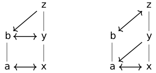
The following, however, are not retraction pairs A \xtofrom [g]{f} B:
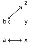
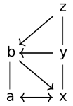
(y \mapsto b \mapsto z but z \not \sqsubseteq y)
(b \mapsto x \mapsto a but a \neq b)
DefinitionComposition of retraction pairs [dt-0056]
We can compose retraction pairs by composing their embedding and projection:

CorollaryDerived products of retraction pairs [dt-0057]
It follows from the definition of retraction pairs that, for a pair \xtofrom [g]{f}:
- f and g are strict, i.e. f(\bot ) = \bot and g(\bot ) = \bot .
- g is uniquely determined by f and vice-versa, so if another retraction pair \xtofrom [g']{f} exists, then g = g'. To see why, remember that f and g must be continuous and therefore monotonic.
- A is isomorphic to the range of f, i.e. A \simeq \{ f(x) \mid x \in A\} \subseteq B.
DefinitionThe category \textbf {Cpo}^\textbf {R} [dt-0058]
The category \textbf {Cpo}^\textbf {R} is the category where the objects are cpos, the morphisms are retraction pairs, composition is as in Definition [dt-0056] and identity is just the retraction pair A \xtofrom [\lambda x. x]{\lambda x. x} A.
DefinitionInformation ordering in \textbf {Cpo}^\textbf {R} [dt-0059]
The third point in Corollary [dt-0057] suggests a notion of approximation, or information ordering, for cpos. Rather than say, as we did in § [dt-004O], that for cpos A and B, A \sqsubseteq B iff there exists a continuous function A\twoheadrightarrow B, we now say:
Generalising to \textbf {Cpo}^\textbf {R} [dt-005A]
All of our other notions for \textbf {Cpo} naturally generalise to a setting with retraction pairs \textbf {Cpo}^\textbf {R}: least elements, \omega -chains, upper bounds, colimits, cocontinuous endofunctors and so on.
Definition\omega -chains of cpos in the category \mathbf {Cpo}^\textbf {R} [dt-005C]
An \omega -chain of cpos in the category \mathbf {Cpo}^\textbf {R} consists of a family of cpos \{D_i \mid i \in \mathbb {N} \}, together with a family of retraction pairs D_i \xtofrom [g_i]{f_i} D_{i+1}, shown below:

DefinitionEndofunctors on \textbf {Cpo}^\textbf {R} [dt-005D]
An endofunctor on the category \textbf {Cpo}^\textbf {R} is a functor \textbf {Cpo}^\textbf {R} \rightarrow \textbf {Cpo}^\textbf {R}, i.e. a mapping \mathcal {F} on cpos together with a mapping \mathcal {F} on retraction pairs, such that:
- If (f,g) is a retraction pair A \xtofrom [g]{f} B then \mathcal {F}(f,g) is a retraction pair \mathcal {F}(A)\xtofrom []{} \mathcal {F}(B)
- \mathcal {F}(\mathsf {id}_A : A\xtofrom []{} A) = \mathsf {id}_{\mathcal {F}(A)} : \mathcal {F}(A)\xtofrom []{} \mathcal {F}(A)
- \mathcal {F}(f \circ g) = \mathcal {F}(f) \circ \mathcal {F}(g) (where \circ is composition of retraction pairs)
DefinitionUpper bounds in the category \mathbf {Cpo}^\mathbf {R} [dt-005G]
A cpo A is an upper bound of an \omega -chain of cpos A_i in the category \mathbf {Cpo}^\textbf {R} if there is a family of retraction pairs A_i \xtofrom [g_i]{f_i} A such that the following diagram commutes (i.e. for all i \in \mathbb {N}, (f_i, g_i) = (f_{i+1},g_{i+1}) \circ (s_i,t_i), where \circ is composition of retraction pairs):
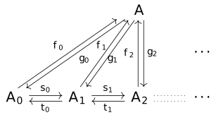
DefinitionColimits in the category \mathbf {Cpo}^\mathbf {R} [dt-005F]
A cpo A is the colimit of an \omega -chain of cpos A_i if is both an upper bound, i.e. there exists retraction pairs (f_i,g_i) : A_i \xtofrom []{} A, and for any other upper bound B, for which there will exist retraction pairs (m_i,n_i) : A_i \xtofrom []{} B, there exists a unique retraction pair A \xtofrom [k']{k} B such that (m_i,n_i) = (k,k') \circ (f_i,g_i) for all i \in \mathbb {N}, where \circ is composition of retraction pairs. Viewed diagramatically, it is the same as Definition [dt-004S] where continuous functions are replaced by retraction pairs.
DefinitionCocontinuous endofunctors on \textbf {Cpo}^\textbf {R} [dt-005E]
An endofunctor \mathcal {F} is cocontinuous iff it preserves colimits of \omega -chains of cpos. That is, given a chain where A is a colimit:
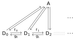
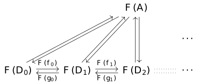
Extending cpo Mappings to endofunctors on \textbf {Cpo}^\mathbf {R} [dt-005I]
If \mathcal {F} is a mapping on cpos built up from basic cpos using the constructions \times , \otimes , +, \oplus , (\cdot )_\bot , as well as \twoheadrightarrow and \mathbin {\circ \hspace{-0.4em}\twoheadrightarrow }, then \mathcal {F} extends to a (covariant!) cocontinuous functor on \textbf {Cpo}^\mathbf {R}. We shall detail the construction for products and functions here, but the other constructions are all similar.
Definition\times operation for retraction pairs [dt-005J]
Given two retraction pairs (f,g) and (h,i), our retraction pair for their product is just the product of their embedding and projection, i.e. (f \times h, g \times i), using our product operation on continuous functions: \dfrac {A \xtofrom [g]{f} B\quad C \xtofrom [i]{h} D}{A\times C \xtofrom [g \times i]{f \times h} B \times D}
Definition\twoheadrightarrow operation for retraction pairs [dt-005K]
We are given two retraction pairs A \xtofrom [g]{f} B and C \xtofrom [i]{h} D. To define a suitable covariant functor, we define our morphism mapping in terms of our \twoheadrightarrow operation on continuous functions: (f,g) \twoheadrightarrow (h,i) \; \triangleq \; (g\twoheadrightarrow h, f \twoheadrightarrow i) Note that the positions of f and g are swapped in the above definition. \dfrac {A \xtofrom [g]{f} B \quad C \xtofrom [i]{h} D}{A \twoheadrightarrow C \xtofrom [f \twoheadrightarrow i]{g \twoheadrightarrow h} B \twoheadrightarrow D} Unlike with the category \textbf {Cpo}, this functor is not contravariant but covariant: Note the positions of A and B are not swapped!
TheoremFixed point theorem for endofunctors on \textbf {Cpo}^\textbf {R} [dt-005B]
Every cocontinuous endofunctor \mathcal {F} on \mathbf {Cpo}^\textbf {R} has a least fixed point, given by the colimit of the ascending \omega -chain:

ConstructionThe colimit D^\infty [dt-005H]
Given an \omega -chain:
The colimit (or inverse limit) is the cpo of \omega -tuples: D_\infty \; \triangleq \; \left \{ (x_0, x_1, \dots ) \mid x_i \in D_i \land x_i = g_i(x_{i+1}) \right \} That is, it is countable sequence of elements, one for each domain D_i, where each element is consistent with earlier elements.
Ordering: The ordering is the pointwise ordering of products, naturally generalised to \omega -tuples. Under this ordering, D_\infty is a cpo. In fact if each D_i is a Scott domain, so is D_\infty .
We shall prove that D_\infty is an upper bound of the \omega -chain. Proof that it is the least upper bound is straightforward but tedious, and is omitted. We must construct a family of retraction pairs:
\left \{ D_i \xtofrom [\theta _{\infty ,i}]{\theta _{i,\infty }} D_\infty \middle |\;\; i \in \mathbb {N}\;\; \right \}
such that the following diagram commutes:
Proof.
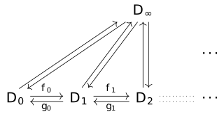
Semantics of untyped \lambda -calculus [dt-005L]
Recall the untyped \lambda calculus:
Untyped \lambda -calculus consists only of untyped (higher-order) functions:
e \; \Coloneqq \; x \mid \lambda x. e \mid e_1\ e_2
DefinitionUntyped \lambda -calculus [dt-004K]


We will now sketch a proof of the retraction pair between D_\infty and D_\infty \twoheadrightarrow D_\infty , by providing two functions, \textbf {\textsf {up}} : D_\infty \rightarrow (D_\infty \twoheadrightarrow D_\infty ) and its inverse \textbf {\textsf {down}} : (D_\infty \twoheadrightarrow D_\infty ) \rightarrow D_\infty .
Observe that each element of D_i (for i > 0) is a function D_{i-1} \twoheadrightarrow D_{i-1}. Therefore, an element of the colimit D_\infty is an \omega -tuple of such functions. To define \textbf {\textsf {up}}(d)(x), we must essentially "apply" each function in the element d \in D_\infty (viewed as an \omega -tuple of functions) to the element x \in D_\infty (viewed as an \omega -tuple of values). More specifically, we say that \textbf {\textsf {up}}(d)(x) is an \omega -tuple (y_m \mid y \in \mathbb {N}), as follows: y_m = \bigsqcup _{k \in \mathbb {N}} \theta _{m+k,m}(d_{m+k+1}(x_{m+k})) To define \textbf {\textsf {down}}(f), we are given a (continuous) function f : D_\infty \twoheadrightarrow D_\infty and must construct the \omega -tuple of approximations at every D_n. We do this by projecting the action of f down to D_n. We say that \textbf {\textsf {down}}(f) is an \omega -tuple (v_n \mid n \in \mathbb {N}) where: \begin {array}{lcl} v_0 & \triangleq & \theta _{\infty ,0}(f(\theta _{0,\infty }(\bot _{D_0})))\\ v_{n+1} & \triangleq & \theta _{\infty ,n} \circ f \circ \theta _{n,\infty } \end {array}
DefinitionDenotations for untyped \lambda -calculus
Using the new functions \textbf {\textsf {up}} and \textbf {\textsf {down}}, it is now straightforward to define a semantics for untyped \lambda -calculus, where \sigma is an environment \mathsf {Var} \rightarrow D_\infty : \llbracket \cdot \rrbracket : (\mathsf {Var} \rightarrow D_\infty )\twoheadrightarrow D_\infty \begin {array}{lcl} \llbracket x \rrbracket \sigma & = & \sigma (x) \\ \llbracket e_0\ e_1 \rrbracket \sigma & = & \textbf {\textsf {up}}(\llbracket e_0 \rrbracket \sigma ) (\llbracket e_1 \rrbracket \sigma )\\ \llbracket \lambda x.\ e \rrbracket \sigma & = & \textbf {\textsf {down}}(\boldsymbol {\lambda } v \in D_{\infty }.\ \llbracket e \rrbracket \ \sigma (x \mapsto v) ) \end {array} This semantics does not distinguish non-terminating computations from terminating ones. To model call-by-value more faithfully, we could use the equation D \simeq D\twoheadrightarrow D_\bot instead, and for call-by-name we could use D \simeq D_\bot \twoheadrightarrow D_\bot . The constructions are very similar.
LectureMonadic semantics, Scott domains and nondeterminism [dt-005V]
This lecture is based on material from Carl Gunter, Glynn Winskel, Graham Hutton, Kai Engelhardt, Dexter Kozen, Andrew Myers, John Longley, Dana Scott, and Joseph Stoy.
Generalising our semantics [dt-005Z]
We return to the \mathcal {C} language we saw previously:
DefinitionThe \mathcal {C} Language [dt-005R]
Using notation similar to Backus-Naur Form (BNF): \begin {array}{lcl} \mathcal {E} & \Coloneqq & n \mid x \mid \mathcal {E}_1 + \mathcal {E}_2 \mid \mathcal {E}_1 - \mathcal {E}_2\\ \mathcal {B} & \Coloneqq & \mathsf {false} \mid \mathsf {true} \mid \neg \mathcal {B} \mid \mathcal {E}_1 = \mathcal {E}_2\\ \mathcal {C} & \Coloneqq & \mathsf {skip} \mid x := \mathcal {E} \mid \mathcal {C}_1 ; \mathcal {C}_2 \mid \mathsf {if}\ \mathcal {B}\ \mathsf {then}\ \mathcal {C}_1\ \mathsf {else}\ \mathcal {C}_2 \mid \mathsf {while}\ \mathcal {B}\ \mathsf {do}\ \mathcal {C}\ \mathsf {od}\\ x & \in & \mathcal {V}\; \textit {(variables)}\\ n & \in & \mathbb {N} \end {array}
If we wish to add other kinds of effects (beyond mutation of state) to our language, this will necessarily affect the semantic domain. Rather than rewrite the entire semantics for each possible setting, we will generalise the semantics to work over any instance of an algebraic structure, called a monad.
DefinitionMonad [dm-000U]
A monad on the category \textbf {C} consists of an endofunctor \mathcal {M} : \textbf {C} \rightarrow \textbf {C} and two operations (natural transformations) for all \mathbf {C}-objects X: \mu _X : \mathcal {M}(\mathcal {M}(X)) \rightarrow \mathcal {M}(X) and \eta _X : X \rightarrow \mathcal {M}(X), such that the following diagrams commute:
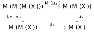
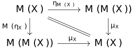
- \mu _X \circ \mathcal {M}(\mu _X) = \mu _X \circ \mu _{\mathcal {M}(X)}
- \mu _X \circ \mathcal {M}(\eta _X) = \mu _X \circ \eta _{\mathcal {M}(X)} = \mathsf {id}_{\mathcal {M}(X)}
ExampleFlat domains as monads [dt-005P]
The flat domain lifting operation (\cdot )_\bot forms a monad, where the endofunctor \mathcal {M}(X) = X_\bot , the operation \mu _X : (X_\bot )_\bot \rightarrow X_\bot collapses the two \bot values, and \eta _X : X \rightarrow X_\bot is simply \eta _X(x) = x.
Sometimes it is more convenient to work with the Kleisli composition operator, rather than the operations \mu and \eta directly.
DefinitionKleisli category [dm-000T]
For a monad (\mathcal {M}, \mu , \eta ) over the category \mathbf {C}, the Kleisli category has the same objects as \mathbf {C}, but the morphisms A \xrightarrow {h} B are those morphisms h of \mathbf {C} that have the form A \xrightarrow {h} \mathcal {M}(B). Composition is defined as follows, for morphisms A \xrightarrow {f} \mathcal {M}(B) and B \xrightarrow {g} \mathcal {M}(C): g \circ _K f = \mu _C \circ \mathcal {M}(g) \circ f Identity morphisms for this category are just \eta .
DefinitionMonadic semantics for \mathcal {C} [dt-005Q]
We define our semantics generically in terms of a monad (\mathcal {M},\mu ,\eta ), using the Kleisli composition operator for \mathcal {M}: \begin {array}{l} \mathsf {ite} : (\Sigma \rightarrow \mathbb {B}) \times (\Sigma \rightarrow \mathcal {M}(\Sigma )) \times (\Sigma \rightarrow \mathcal {M}(\Sigma )) \rightarrow (\Sigma \rightarrow \mathcal {M}(\Sigma ))\\ \mathsf {ite}(b,t,e)(\sigma ) = \begin {cases}t(\sigma ) & \text {if}\ b(\sigma ) = T \\ e(\sigma ) & \text {otherwise} \end {cases} \end {array} \begin {array}{lcl} \llbracket \cdot \rrbracket _\mathcal {C} : \mathcal {C} \rightarrow \Sigma \rightarrow \mathcal {M}(\Sigma )\\[0.4em] \llbracket \mathsf {skip} \rrbracket _\mathcal {C} & = & \eta _\Sigma \\ \llbracket x := e \rrbracket _\mathcal {C} & = & \boldsymbol {\lambda } \sigma .\ \eta _\Sigma (\sigma \left (x \mapsto \llbracket e \rrbracket _\mathcal {E}\right )) \\ \llbracket c_1 ; c_2 \rrbracket _\mathcal {C} & = & \llbracket c_2 \rrbracket _\mathcal {C} \circ _K \llbracket c_1 \rrbracket _\mathcal {C} \\[0.3em] \llbracket \textsf {if}\ b\ \textsf {then}\ c_1\ \textsf {else}\ c_2 \rrbracket _\mathcal {C} & = & \mathsf {ite}(\llbracket b \rrbracket _\mathcal {B},\llbracket c_1 \rrbracket _\mathcal {C},\llbracket c_2 \rrbracket _\mathcal {C})\\ \llbracket \textsf {while}\ b\ \textsf {do}\ c\ \textsf {od} \rrbracket _\mathcal {C} & = & \mathbf {\mathbf {fix}}(\boldsymbol {\lambda } f.\ \mathsf {ite}(\llbracket b \rrbracket _\mathcal {B}, f \circ _K \llbracket c \rrbracket _\mathcal {C}, \eta _\Sigma ) ) \end {array}
ExampleInstantiating \mathcal {C} with the lifting monad [dt-005S]
Instantiating our monadic semantics where the monad \mathcal {M} is flat domain lifting, we recover our original semantics of \mathcal {C}.
ExampleInstantiating \mathcal {C} with exceptions [dt-005T]
Let us instantiate our monadic semantics with the monad \mathcal {M}(X) = X_\bot \oplus \mathbf {1}, where the added value (from \mathbf {1}) is called \mathsf {fail}. The operation \mu _X : (X_\bot \oplus \mathbf {1})_\bot \oplus \mathbf {1} \rightarrow X_\bot \oplus \mathbf {1} collapses the two possible \bot values to \bot and the two possible \mathsf {fail} values to \mathsf {fail}, and the operation \eta _X : X \rightarrow X_\bot \oplus \mathbf {1} is the straightforward injection.
Then we may extend our language with lightweight exception constructs: \mathcal {C} ::= \dots \mid \mathsf {throw} \mid \mathsf {try}\ \mathcal {C}_1\ \mathsf {catch}\ \mathcal {C}_2 and define their semantics, leaving our existing semantics unchanged: \begin {array}{lcl} \llbracket \mathsf {throw} \rrbracket \ \sigma &=& \mathsf {fail} \\ \llbracket \mathsf {try}\ c_1\ \mathsf {catch}\ c_2 \rrbracket \ \sigma &=& \begin {cases} \llbracket c_2 \rrbracket \ \sigma & \text {if}\ \llbracket c_1 \rrbracket \ \sigma = \mathsf {fail} \\ \llbracket c_1 \rrbracket \ \sigma & \text {otherwise}\end {cases} \end {array}
Nondeterminism
Introduction to nondeterminism [dt-005U]
When modelling programming languages we sometimes require a way to be imprecise about some aspects of a program — usually, this takes the form of non-determinism. Non-determinism can be hard for beginners to grasp, but it typically has to be employed when modelling real programs. For example, suppose we had a greeting program that differed depending on the physical location of the computer: \begin {array}{l} \textsf {\textbf {if}}\ \mathit {currentLocation}() = \text {Korea}\ \textsf {\textbf {then}} \\ \quad \textsf {\textbf {say}}\ \text {``안녕하세요''} \\ \textsf {\textbf {else}} \\ \quad \textsf {\textbf {say}}\ \text {``Hello!''}\\ \textsf {\textbf {fi}} \end {array} If we wanted to mathematically model the behaviour of this program, it would be frightfully inconvenient to include the geography of Earth and the computer's physical location in our model. That's where non-determinism comes in. If we abstract away from the geographical details, and instead regard the program as choosing between the two options based on some unspecified criteria, then we can get away with modelling less, at the cost of some detail: \begin {array}{l} \textsf {\textbf {if}}\ \mathit {???}\ \textsf {\textbf {then}} \\ \quad \textsf {\textbf {say}}\ \text {``안녕하세요''} \\ \textsf {\textbf {else}} \\ \quad \textsf {\textbf {say}}\ \text {``Hello!''}\\ \textsf {\textbf {fi}} \end {array} Such underspecified conditionals are usually called non-deterministic choice, where our conditional \textsf {\textbf {if}}\ \mathit {???}\ \textsf {\textbf {then}}\ P\ \textsf {\textbf {else}}\ Q\ \textsf {\textbf {fi}} is written simply as P + Q.
While we tend to view our physical machines as deterministic automata, the state upon which each decision is deterministically made includes a number of external things which are tedious to model mathematically. We can also use non-determinism to ignore details that we don't care about for our particular domain — a common example is memory allocation, where it is very convenient (for some programs) to think of memory as infinite, and allocation as an operation that can potentially fail, without specifying exactly when and how this failure can occur. This is normally modelled as a choice between successful allocation and a failure state.
Instantiating our semantics for nondeterminism [dt-0060]
Our initial semantics for \mathcal {C} (without loops) was functions on states \Sigma \rightarrow \Sigma . When adding loops, we used a cpo \Sigma \twoheadrightarrow \Sigma _\bot for our semantic domain. Since non-deterministic programs can have more than one outcome, a natural choice of semantic domain would be \Sigma \twoheadrightarrow \mathcal {P}(\Sigma _\bot ) \setminus \emptyset , i.e., functions from an initial state to a non-empty set of possible outcomes.
We can provide \eta and \mu operations for our proposed monad for non-determinism \mathcal {M}(X) = \mathcal {P}(X_\bot ) \setminus \emptyset : \begin {array}{l} \eta : X \rightarrow \mathcal {P}(X_\bot ) \setminus \emptyset \\ \eta (x) = \{ x \}\\ \mu : \mathcal {P}{((\mathcal {P}(X_\bot ) \setminus \emptyset )_\bot )}\rightarrow \mathcal {P}(X_\bot ) \setminus \emptyset \\ \mu (S) = (\bigcup _{X \neq \bot \in S} X) \cup (S \cap \{ \bot \}) \end {array} And, with this semantics, we can easily add a denotation for a non-deterministic choice operator, in terms of union: \llbracket c_1 + c_2 \rrbracket _\mathcal {C} = \lambda \sigma . \llbracket c_1 \rrbracket _\mathcal {C} \sigma \cup \llbracket c_2 \rrbracket _\mathcal {C} \sigma Unfortunately this is only the beginning of our troubles. While we have given a valuation function above, its definition uses \textbf {fix}, and therefore our domain \Sigma \rightarrow \mathcal {M}(\Sigma ) must be a cpo, and all our operations continuous. It is not clear how to order elements of \mathcal {P}(X_\bot ) \setminus \emptyset . A natural choice of ordering would be subset inclusion \subseteq . However, as we lack \emptyset , there is no least element for this ordering. Furthermore, simply using \subseteq as our ordering would mean that the deterministic, terminating program that always returns a single state \{ \sigma \} would be considered less informative than the program that may diverge \{ \bot , \sigma \}. This would make most of our operations non-continuous.
Instead, we shall examine three separate orderings on this set, each of which carries a different view of non-determinism. More generally, we wish to come up with a construction analogous to the powerset operator \mathcal {P}, but for our semantic domains — a powerdomain. However, for these orderings to produce valid partial orders, we require a certain theorem that only applies to a certain class of cpos, called "algebraic" cpos. Thus, we will first introduce a richer class of cpos, called Scott domains, and then return to the problem of non-determinism.
Scott domains [dt-005W]
Compactness and Finiteness [dt-0040]
We begin by formalising the notion of an element in a cpo representing a finite amount of information.
DefinitionBoring and interesting sets [dt-003W]
There are two kinds of directed sets:
Following the above intuition, we might be tempted to say that the "infinite" elements of a cpo are those which are the lub of an interesting set, but this notion is too weak. Consider this cpo X:
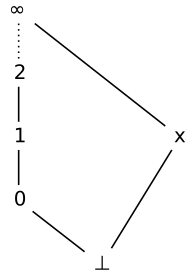
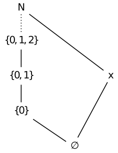
DefinitionCompactness [dt-003U]
Let A be a cpo. Then x \in A is compact (a.k.a. finite) iff for all directed X \subseteq A: x \sqsubseteq \bigsqcup X \implies \exists y \in X.\ x \sqsubseteq y In English: A compact element will approximate some element of a directed set if it approximates the lub. We write \mathsf {K}(A) for the set of compact elements of A, i.e.: \mathsf {K}(A) = \{x \in A \mid x\ \text {is compact} \}
In the example cpo X above, all the elements except \infty and x would be compact. Thus, compactness better captures our notion of an element representing a finite amount of information. This understanding of compact elements is a generalisation of the notion of a finite element from the theory of algebraic lattices.
ExampleCompact elements [dt-003V]
- Every element in a finite cpo is compact. More generally, every element of a cpo of finite height (e.g. \mathbb {Z}_\bot ) is compact. This is because finite directed sets are always boring.
- Take the cpo \mathcal {P}(X) of subsets of X ordered by inclusion \subseteq , as seen in Exercise [dt-001G]. The compact elements of \mathcal {P}(X) are those of finite cardinality.
- Take the cpo \mathbb {N} \nrightarrow \mathbb {N} of partial functions on the natural numbers, ordered by inclusion of graphs. The compact elements of \mathbb {N} \nrightarrow \mathbb {N} are the functions which are defined only for finite domains.
ExampleCompact elements with infinitely many approximations [dt-003X]
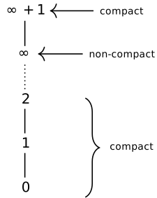
Compact elements may still have an infinite number of approximations. Consider the cpo \mathbb {N} \cup \{ \infty , \infty + 1 \}, where we have tacked on an additional top element \infty + 1 to our normal cpo of natural numbers extended with infinity. Then, while \infty is not compact, \infty + 1 is compact — it is not the lub of an interesting directed set. If \infty + 1 is the lub of a set X then \infty + 1 must be in the set X. Nonetheless, there are an infinite number of approximations to \infty + 1, i.e., elements x such that x \sqsubseteq \infty + 1.
As an aside, requiring that our compact elements have a truly finite number of approximations is the basis for the theory of Berry domains and stable functions.
TheoremSubmonoids as a cpo [dt-003Y]
The submonoids of a monoid (X, \iota , \bullet ) form a cpo under \subseteq , where union gives the lub.
ExerciseBoth infinite and compact [dt-003Z]
Find a set in the cpo of submonoids of (\mathbb {N},0,+) that is both infinite and compact.
Solution.
Take E \triangleq \{ n \in \mathbb {N} \mid n\ \text {is even}\}. Let Y \subseteq \mathcal {P}(\mathbb {N}) be directed and E \subseteq \bigcup Y. Since 2 \in E there must exist y \in Y such that 2 \in Y. Since (y,0,+) is a monoid, every positive multiple of 2 is also in y, thus E \subseteq y and therefore E is compact.
Seeing as compact elements are also sometimes called finite, this is surprising as E is an infinite set. The reason it is nonetheless compact is that E is finitely generated — it is the smallest submonoid of (\mathbb {N},0,+) such that the finite set \{ 2 \} \subseteq E. In fact, the compact submonoids of (\mathbb {N},0,+) are precisely the finitely generated ones.
Algebraicity and ideals [dt-005X]
DefinitionAlgebraicity [dt-0041]
A cpo is algebraic iff every element is the lub of its compact approximations. That is, a cpo D is algebraic iff for all x \in D,
- \mathop {\downarrow }(x) = \{ y \in \mathsf {K}(D) \mid y \sqsubseteq x \} is directed;
- x = \bigsqcup \mathop {\downarrow }(x)
Aside: Plotkin provides an equivalent definition of \omega -algebraic cpos in which directed sets are replaced with \omega -chains throughout. Hutton claims this is less appealing, as the definition speaks of an \omega -chain of compact approximations, rather than the directed set of such.
Example\omega -algebraic cpos [dt-0042]
Many standard examples of cpos are \omega -algebraic cpos: finite cpos, subsets \mathcal {P}(X) of a set X, partial functions \mathbb {N} \nrightarrow \mathbb {N} and submonoids of a monoid. In general, any cpo of subalgebras (e.g. subgroups of a group, subrings of a ring etc.) is \omega -algebraic. This is the origin of the terminology.
CounterexampleNon-algebraic cpo [dt-0043]
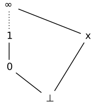
In the cpo on the right (seen also in § [dt-0040]), the element x is not the lub of its compact approximations. The only compact element that approximates x is \bot , and the least upper bound of the set \{\bot \} is just \bot , not x. That is: \mathop {\downarrow }(x) = \{\bot \} but: x \neq \bigsqcup \{\bot \}
TheoremNothing suddenly invented at infinity [dt-0045]
Let D and E be algebraic cpos. Then a function f : D \rightarrow E is continuous iff, for all x \in D: f(x) = \bigsqcup \ \{ f(a) \mid a \in \mathop {\downarrow }(x) \} In other words, in an algebraic cpo, continuous functions are completely defined by their behaviour for compact arguments.
This makes precise our earlier slogan in Definition [dt-001J], that continuous functions don't suddenly behave differently for infinite (i.e. non-compact) elements.
Proof.
Exercise [dt-0044]
Let f : D \twoheadrightarrow E be a continuous function between algebraic cpos. Define: G_f = \{ (a,b) \in \mathsf {K}(D) \times \mathsf {K}(E) \mid b \sqsubseteq f(a) \} Then for all x \in D, prove that: f(x) = \bigsqcup \ \{ b \mid (a,b) \in G_f \land a \sqsubseteq x \}
Solution.
This is powerful. For example, the continuous function f : \mathcal {P}(\mathbb {N}) \twoheadrightarrow \mathcal {P}(\mathbb {N}) on an uncountable cpo \mathcal {P}(\mathbb {N}) is completely determined by the countable relation G_f.
DefinitionDown-closure [dt-0047]
Given a poset Y, a set X \subseteq Y is down-closed iff, for all x \in X, any y \sqsubseteq x is in X.
DefinitionIdeal [dt-0048]
A set is ideal iff it is both down-closed and directed.
DefinitionIdeal completion [dt-0046]
The ideal completion of a set A, written sometimes as \mathsf {Id}(A), is the set of all ideal subsets of A, i.e.: \mathsf {Id}(A) = \{ X \subseteq A \mid X\ \text {is ideal}\}
TheoremRepresentation theorem for algebraic cpos [dt-0049]
Every algebraic cpo D is isomorphic to the ideal completion of its compact elements, ordered by subset inclusion. That is, \mathsf {Id}(K(D)) is an algebraic cpo such that D \simeq \mathsf {Id}(K(D)) .
Getting closure [dt-005Y]
DefinitionBasis [dt-004A]
TheoremCompact basis for algebraic cpos [dt-004B]
If X is a basis for A, then A is algebraic and \mathsf {K}(A) = X.
Proof.
If a \in \mathsf {K}(A), then \bigsqcup M = a where M = \{ x \in X \mid x \sqsubseteq a \}, as X is a basis. Since a is compact, a \sqsubseteq b for some b \in M. But since a is the lub of M, b \sqsubseteq a as well. By antisymmetry a = b, hence a \in X. Thus \mathsf {K}(A) \subseteq X, so \mathsf {K}(A) = X and A is algebraic.
TheoremClosure of algebraic cpos under product [dt-004C]
If D and E are algebraic cpos, then so is their product construction D \times E.
Proof.
In the following proof, we show that \mathsf {K}(D) \times \mathsf {K}(E) is a basis for the product D \times E and thereby show via Theorem [dt-004B] that D \times E is algebraic if D and E are.
- \mathsf {K}(D) \times \mathsf {K}(E) \subseteq \mathsf {K}(D \times E): Let (x,y) \in \mathsf {K}(D) \times \mathsf {K}(E). To show that (x,y) is compact, let us assume that (x,y) \in \bigsqcup X where X \subseteq D \times E is directed. We must show that there exists some element e of X such that our (x,y) \sqsubseteq e. As (x,y) \in \bigsqcup X, by the definition of lub on products we can conclude that:
\begin {array}{lcl}
x & \sqsubseteq & \bigsqcup \pi _0[ X] \\
y & \sqsubseteq & \bigsqcup \pi _1[X]
\end {array}
Here we use the notation f[X] to indicate the image of a function on a set, i.e. \{ f(v) \mid v \in X \}.
Since x and y are both compact, there must exist x' \in \pi _0[ X] and y' \in \pi _1[ X] such that x \sqsubseteq x' and y \sqsubseteq y'. While it does not follow that (x', y') \in X, we know that there must exist a pair (a,b) \in X such that x' \sqsubseteq a and y' \sqsubseteq b as X is directed. Hence (a,b) can be our element e \in X that is approximated by (x,y), i.e. (x,y) \sqsubseteq (a,b). - \mathop {\downarrow }(x,y) is directed for all (x,y) \in D \times E: \begin {array}{lcl} \mathop {\downarrow }(x,y) &= & \{ (a,b) \in \mathsf {K}(D) \times \mathsf {K}(E) \mid (a,b) \sqsubseteq (x,y) \} \\ & = & \{ a \in \mathsf {K}(D) \mid a \sqsubseteq x \} \times \{ b \in \mathsf {K}(E) \mid b \sqsubseteq y \}\\ & = & \mathop {\downarrow }(x) \times \mathop {\downarrow }(y) \end {array} Because D and E are algebraic, \mathop {\downarrow }(x) and \mathop {\downarrow }(y) are directed. As directedness is closed under product, \mathop {\downarrow }(x,y) is directed too.
- (x,y) = \bigsqcup \mathop {\downarrow }(x,y) Starting from the right hand side: \begin {array}{lclr} \bigsqcup \mathop {\downarrow }(x,y) & = & \bigsqcup (\mathop {\downarrow }(x) \times \mathop {\downarrow }(y)) & \text {(part 2)}\\ & = & (\bigsqcup (\mathop {\downarrow }(x), \bigsqcup \mathop {\downarrow }(y))) & \text {(lub on products)}\\ & = & (x,y) & \text {($D$, $E$ are {algebraic})} \end {array}
Problem.
AsideScott's original solution: using complete lattices [dt-004D]
The lack of closure of algebraicity under the (continuous) function arrow, strict or non-strict, is not satisfying as it means that our semantic domains are not guaranteed to be algebraic even if they are composed from algebraic cpos. Instead, we must replace algebraic cpos with something stronger still.
Scott's original solution to this lack of closure was to use a complete lattice instead of cpos, i.e. requiring lubs for all subsets, not just directed ones. This solves the problem with \twoheadrightarrow but introduces new problems:
- Complete lattices need a top element \top , but adding a fictitious top (representing inconsistent information) to cpos like \mathbb {B}_\bot is strange.
- Extending the functions that capture our primitive semantic operations to complete lattices can spoil nice algebraic properties. Consider these two possible implementations of \mathsf {ite}, the function for the semantics of an \mathsf {if} expression: \mathsf {ite}(\top ,x,y) = x \sqcup y\quad \quad \quad \quad \quad \mathsf {ite}(\top ,x,y) = \top Either of these solutions results in the failure of useful and expected laws for \mathsf {if} expressions. For example, the left definition above results in the failure of the common equation to eliminate unreachable cases: \mathsf {ite}(b, \mathsf {ite}(b,x,y),z) = \mathsf {ite}(b,x,z) And the second definition above results in the failure of this equation that removes redundant checks: \mathsf {ite}(b,x,x) = x
- The powerdomain construction does not generalise to complete lattices, so semantics for non-deterministic programs are difficult in this setting.
DefinitionConsistent completeness [dt-004E]
A poset A is consistent complete (or bounded complete) iff \bigsqcup X exists for all consistent X \subseteq A. That is, any set with an upper bound (a consistent set) has a least upper bound.
ExampleConsistent completeness vs directed completeness [dt-004F]

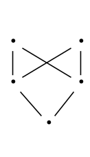
DefinitionScott domain [dt-004G]
A cpo D is a Scott domain iff:
- D is \omega -algebraic,
- D is consistent complete,
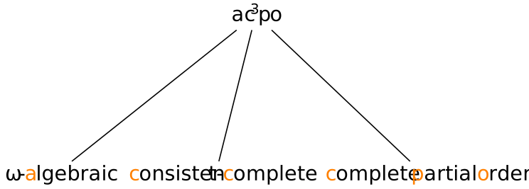
Remark [dt-004H]
The second requirement in Definition [dt-004G] can, in light of the first, be expressed equivalently as: x \sqcup y exists for all consistent x,y \in D. This is useful when needing to show that a given cpo is a Scott domain.
TheoremClosure of Scott domains [dt-004I]
Scott domains are closed under all our cpo constructions, including sums +, products \times , continuous functions \twoheadrightarrow , smash sums \oplus , smash products \otimes and strict functions \mathbin {\circ \hspace{-0.4em}\twoheadrightarrow }.
Thesis.
Our semantic domains are Scott domains.
The Hoare powerdomain [dt-0061]
We write \mathcal {P}_f^\ast (S) to denote finite non-empty subsets of S. Let X, Y \in \mathcal {P}_f^\ast (\mathsf {K}(A)) be finite, non-empty sets of compact elements of a Scott domain A. The Hoare powerdomain construction is based on the following ordering: X \preceq _H Y\quad \text {iff}\quad (\forall x \in X.\ \exists y \in Y.\ x \sqsubseteq _A y) The intuition behind this is that "Anything X can do, Y can do better". This ordering has some desirable properties: The least element is \{\bot \}, as we might expect. It also satisfies the equation X \preceq _H X \cup Y, which intuitively means that a non-deterministic choice is considered to have more information than any of its components. When specialised to the case where A is a flat domain like \Sigma _\bot , it simplifies to: X \preceq _H Y\quad \text {iff}\quad X \setminus \{\bot \} \subseteq Y This is, however, not a proper order, but a preorder, as it fails antisymmetry. Even in the flat domain case, \{ x, \bot \} \preceq _H \{x \} and \{ x \} \preceq _H \{x, \bot \} but they are not equal. However, any preorder does induce an equivalence relation, where X \approx _H Y iff X \preceq _H Y and Y \preceq _H X. Furthermore, if we take the ideal completion of \mathcal {P}_f^\ast (K(A)) with respect to the preorder \preceq _H (i.e., the set of all \preceq _H-downwards-closed directed subsets of \mathcal {P}_f^\ast (\mathsf {K}(A))), we can order them by inclusion to obtain an algebraic domain with compact elements which correspond to equivalence classes of elements under \approx _H. We have a lub operation for these ideals: A \sqcup _H B = \{ X \cup Y \mid X \in A \land Y \in B \}
ExampleHoare powerdomain of \mathbb {N}_\bot [dt-0062]
Let us find the Hoare powerdomain of \mathbb {N}_\bot . Note that \mathbb {N}_\bot is a flat domain so all elements are compact, i.e. \mathsf {K}(\mathbb {N}_\bot ) = \mathbb {N}_\bot . Let us find examine the \preceq _H-ideal subsets of \mathcal {P}_f^\ast (\mathbb {N}_\bot ). If v and u both contain \bot , then v \preceq _H u iff v \subseteq u. As ideal subsets are downwards closed, we can identify an ideal I \in \mathsf {Id}({\mathcal {P}_f^\ast (\mathbb {N}_\bot )}) with its union \bigcup I. The ideals of \mathcal {P}^\ast _f(\mathbb {N}_\bot ) are then isomorphic to domain \mathcal {P}(\mathbb {N}) of all subsets of \mathbb {N} under subset inclusion.
RemarkAngelic nondeterminism [dt-0063]
Consider the following three programs:
- x := 1
- \textsf {while}\ \textsf {true}\ \textsf {do}\ \textsf {skip}
- \textsf {while}\ \textsf {true}\ \textsf {do}\ \textsf {skip}\ \textsf {od} + x := 1
The Smyth powerdomain [dt-0064]
As before, let X, Y \in \mathcal {P}_f^\ast (\mathsf {K}(A)) be finite, non-empty sets of compact elements of a Scott domain A. The Smyth powerdomain construction is based on the following preorder: X \preceq _S Y\quad \text {iff}\quad (\forall y \in Y.\ \exists x \in X.\ x \sqsubseteq _A y) The intuition here is "Everything Y can do, X can do worse". It satisfies the equation X \cup Y \preceq _S X, which intuitively means that a non-deterministic choice is considered to have less information than any of its components. When applied to a flat domain, it simplifies to: X \preceq _S Y\quad \text {iff}\quad \bot \in X \lor Y \subseteq X As with the Hoare powerdomain, this fails to be a partial order, but we can use the same ideal completion trick to induce an algebraic domain where compact elements correspond to equivalence classes of elements under \approx _S (where X \approx _S Y is, as with \approx _H, just defined as X \preceq _S Y \land Y \preceq _S X).
ExampleSmyth powerdomain of \mathbb {N}_\bot [dt-0065]
Firstly note that, as ideals are downwards-closed, any \preceq _S-ideal subsets of \mathcal {P}^\ast _f(\mathbb {N}_\bot ) will contain all finite subsets of \mathbb {N}_\bot that contain \bot . Let us call those sets trivial. So, a set in \mathcal {P}^\ast _f(\mathbb {N}_\bot ) is non-trivial if it does not contain \bot and an ideal subset of \mathcal {P}^\ast _f(\mathbb {N}_\bot ) is non-trivial if it contains a non-trivial set. Observe that for non-trivial sets X and Y, X \preceq _S Y iff X \supseteq Y. Thus, we can identify an ideal I \in \mathsf {Id}({\mathcal {P}_f^\ast (\mathbb {N}_\bot )}) with the down-closure of the intersection of its non-trivial elements. The smaller this set is, the larger the ideal I. Hence, and confusingly, the non-trivial ideals in the powerdomain (ordered by subset inclusion) correspond to finite subsets of \mathbb {N} ordered by superset inclusion. As all trivial sets are identified, we just need to throw in the unique trivial ideal, and we can see that the Smyth powerdomain of \mathbb {N} is isomorphic to the domain of sets \{ \mathbb {N} \} \cup \mathcal {P}_f^\ast (\mathbb {N}) ordered by subset inclusion.
RemarkDemonic nondeterminism [dt-0066]
Note that all sets that contain \bot are considered equivalent by the Smyth construction \approx _S. Thus, this models demonic non-determinism: Of the three programs in Remark [dt-0063], the Smyth semantics considers 2 and 3 to be the same. Thus, the possibility of divergence \bot is no different from inevitable divergence.
The Plotkin powerdomain [dt-0067]
As before, let X, Y \in \mathcal {P}_f^\ast (\mathsf {K}(A)) be finite, non-empty sets of compact elements of a Scott domain A. The Plotkin powerdomain construction is based on the following preorder, simply combining the orderings from the Hoare and Smyth constructions: X \preceq _P Y\quad \text {iff}\quad X \preceq _H Y \land X \preceq _S Y This ordering is also called the Egli-Milner ordering. On a flat domain, it simplifies to: A\sqsubseteq B\quad \text {iff}\quad A = B \lor (\bot \in A \land (A \setminus \{\bot \})\subseteq B) Note that this is antisymmetric in the case of a flat domain, and the lub of a chain of sets can be found by taking the union of all elements of the chain if all elements contain \bot If not, then the element without \bot will be the least upper bound.
The failures of antisymmetry can only be observed in domains of height higher than one. Consider a set \{x,y\} containing two elements. According to the induced equivalence from this preorder \approx _P, this set would be considered equal to the set that contains those two elements plus any elements that lie between them on the information ordering: \{x,y\} \approx _P \{ z \mid x \sqsubseteq z \sqsubseteq y \} The Plotkin powerdomain is sometimes called the convex powerdomain, due to the similarity of this to the geometric definition of convexity. Thus, we use the ideal completion trick (as with the Hoare and Smyth constructions) here to arrive at a definition of powerdomain that distinguishes between all three programs outlined in Remark [dt-0063].
Aside.
There is a beautiful algebraic characterisation of Plotkin powerdomains in Matthew Hennessy Gordon Plotkin's paper, Full abstraction for a simple parallel programming language.