Lecture. Domain theory › Semantics and recursion [dt-0005]
This lecture is based on material from Graham Hutton, Dana Scott, Joseph Stoy, Carl Gunter, and Glynn Winskel.
Denotational semantics [dt-0003]
In this course we are concerned with programming languages, which, as with natural languages, consist of a syntax and semantics. The syntax of a language is, for our purposes, merely an inductively-defined tree structure (i.e. abstract syntax).
DefinitionThe \mathcal {C} Language (without loops) [dt-0000]
Using notation similar to Backus-Naur Form (BNF): \begin {array}{lcl} \mathcal {E} & \Coloneqq & n \mid x \mid \mathcal {E}_1 + \mathcal {E}_2 \mid \mathcal {E}_1 - \mathcal {E}_2\\ \mathcal {B} & \Coloneqq & \mathsf {false} \mid \mathsf {true} \mid \neg \mathcal {B} \mid \mathcal {E}_1 = \mathcal {E}_2\\ \mathcal {C} & \Coloneqq & \mathsf {skip} \mid x := \mathcal {E} \mid \mathcal {C}_1 ; \mathcal {C}_2 \mid \mathsf {if}\ \mathcal {B}\ \mathsf {then}\ \mathcal {C}_1\ \mathsf {else}\ \mathcal {C}_2\\ x & \in & \mathcal {V}\; \textit {(variables)}\\ n & \in & \mathbb {N} \end {array}
In the language above, there are three syntactic classes: \mathcal {E}, \mathcal {B}, and \mathcal {C}.
DefinitionDenotational semantics [dt-0001]
A denotational semantics consists of, for each syntactic class \mathcal {X} in a language:
- A semantic domain D which can be any set of mathematical objects (although, as we will see later, it is helpful if it obeys certain properties).
- A valuation function \llbracket \cdot \rrbracket : \mathcal {X} \rightarrow D. We require that this function be a homomorphism, that is that it is compositional. This means that the valuation (or denotation) of an expression should be made from the denotation of its components. In other words, for each syntactic constructor C(e_1,e_2,\dots ), we should have a mathematical operation f(x_1,x_2,\dots ) such that the denotation of C can be defined as: \llbracket C(e_1, e_2, \dots ) \rrbracket = f(\llbracket e_1 \rrbracket , \llbracket e_2 \rrbracket , \dots )
Remark [dt-0002]
The choices of semantic domain and valuation function are, essentially, arbitrary: we choose objects that reflect those aspects of our programs that we are interested in. For most of the simple languages we will examine, we are only concerned with the results of the computation, which is a semantics suitable for reasoning about program behaviour and correctness. However, there also exist denotational cost models that compositionally assign a measure of program performance to syntax. This measure is just another kind of denotational semantics.
ExampleDenotational semantics for the \mathcal {C} language (without loops) [dt-0004]
We shall first select a semantic domain for each syntactic class: \begin {array}{lcl} \mathbf {E} & \triangleq & \Sigma \rightarrow \mathbb {Z} \\ \mathbf {B} & \triangleq & \Sigma \rightarrow \mathbb {B} \\ \mathbf {C} & \triangleq & \Sigma \rightarrow \Sigma \\ \end {array} Here, \Sigma represents the set of states, which contains the values assigned to all variables: \Sigma \;\triangleq \; \mathcal {V} \rightarrow \mathbb {Z}
Now, we define our valuation functions, \llbracket \cdot \rrbracket _\mathcal {E} : \mathcal {E} \rightarrow \mathbf {E} : \begin {array}{lcl} \llbracket n \rrbracket _\mathcal {E}\ \sigma & = & n \\ \llbracket x \rrbracket _\mathcal {E}\ \sigma & = & \sigma (x) \\ \llbracket e_1 + e_2 \rrbracket _\mathcal {E}\ \sigma & = & \llbracket e_1 \rrbracket _\mathcal {E}\ \sigma + \llbracket e_2 \rrbracket _\mathcal {E}\ \sigma \\ \llbracket e_1 - e_2 \rrbracket _\mathcal {E}\ \sigma & = & \llbracket e_1 \rrbracket _\mathcal {E}\ \sigma - \llbracket e_2 \rrbracket _\mathcal {E}\ \sigma \\[2em] \end {array} and \llbracket \cdot \rrbracket _\mathcal {B} : \mathcal {B} \rightarrow \mathbf {B}: \begin {array}{lcl} \llbracket \mathsf {false} \rrbracket _\mathcal {B}\ \sigma & = & \mathit {F} \\ \llbracket \mathsf {true} \rrbracket _\mathcal {B}\ \sigma & = & \mathit {T} \\ \llbracket \neg b \rrbracket _\mathcal {B}\ \sigma & = & \begin {cases}\mathit {F} & \text {if}\ \llbracket b \rrbracket _\mathcal {B}\ \sigma = \mathit {T} \\ \mathit {T} & \text {otherwise} \end {cases} \\[1.1em] \llbracket e_1 = e_2 \rrbracket _\mathcal {B}\ \sigma & = & \begin {cases}\mathit {T} & \text {if}\ \llbracket e_1 \rrbracket _\mathcal {E}\ \sigma = \llbracket e_2 \rrbracket _\mathcal {E}\ \sigma \\ \mathit {F} & \text {otherwise} \end {cases} \end {array} and \llbracket \cdot \rrbracket _\mathcal {C} : \mathcal {C} \rightarrow \mathbf {C}: \begin {array}{lcl} \llbracket \mathsf {skip} \rrbracket _\mathcal {C}\ \sigma & = & \sigma \\ \llbracket x := e \rrbracket _\mathcal {C}\ \sigma & = & \sigma \left (x \mapsto \llbracket e \rrbracket _\mathcal {E}\right ) \\ \llbracket c_1 ; c_2 \rrbracket _\mathcal {C}\ \sigma & = & \llbracket c_2 \rrbracket _\mathcal {C}\ \left (\llbracket c_1 \rrbracket _\mathcal {C}\ \sigma \right ) \\[0.3em] \llbracket \textsf {if}\ b\ \textsf {then}\ c_1\ \textsf {else}\ c_2 \rrbracket _\mathcal {C}\ \sigma & = & \begin {cases}\llbracket c_1 \rrbracket _\mathcal {C}\ \sigma & \text {if}\ \llbracket b \rrbracket _\mathcal {B}\ \sigma = \mathit {T} \\ \llbracket c_2 \rrbracket _\mathcal {C}\ \sigma & \text {otherwise} \end {cases} \end {array}
Recursion [dt-000L]
So far, our semantic domains have just been (functions of) sets. While these have the advantage of being mathematically simple and intuitive, two language features make these sets insufficient for our purposes:
- Recursively defined programs, for dealing with recursion and loops, and
- Recursively defined semantic domains, for dealing with higher-order programs.
Recursively defined programs [dt-0006]
Suppose we extended the \mathcal {C} language with a while loop construct: \mathcal {C}\; \Coloneqq \; \cdots \mid \mathsf {while}\ \mathcal {B}\ \mathsf {do}\ \mathcal {C}\ \mathsf {od} The intuitive way to assign a semantics would be to use a recursive function: \llbracket \mathsf {while}\ b\ \mathsf {do}\ c\ \mathsf {od} \rrbracket _\mathcal {C}\ \sigma \; = \; \begin {cases} \llbracket \mathsf {while}\ b\ \mathsf {do}\ c\ \mathsf {od} \rrbracket _\mathcal {C}\ (\llbracket c \rrbracket _\mathcal {C}\ \sigma ) & \text {if}\ \llbracket b \rrbracket _\mathcal {B}\ \sigma = \mathit {T} \\ \sigma & \text {otherwise} \end {cases} However, such an equation is not a good definition. If we consider the trivial infinite loop program L \triangleq \mathsf {while}\ \mathsf {true}\ \mathsf {do}\ \mathsf {skip}\ \mathsf {od}, and compute its semantics, we end up with: \llbracket \mathsf {while}\ \mathsf {true}\ \mathsf {do}\ \mathsf {skip}\ \mathsf {od} \rrbracket _\mathcal {C}\ \sigma \; = \; \llbracket \mathsf {while}\ \mathsf {true}\ \mathsf {do}\ \mathsf {skip}\ \mathsf {od} \rrbracket _\mathcal {C}\ \sigma This equation is satisfied by any function \Sigma \rightarrow \Sigma , so it doesn't tell us which function corresponds to the program L.
More generally, allowing our functions to be (generally) recursive causes these issues. The loop program L gives rise to the recursive equation \ell (x) = \ell (x), which has an infinite number of solutions.
If we add recursion to our programming language, we could have programs that give rise to more complex recursive equations like f(x) = f(x) + 1. By contrast to \ell (x), f(x) has no solutions (assuming f(x) operates on integers).
Upshot.
We need an explicit notion of "non-termination" on the semantics level, to properly deal with general recursion (or iteration).
Recursively defined semantic domains [dt-0007]
Suppose we extend our notion of expressions in the \mathcal {C} language with parameterless higher-order procedures: \begin {array}{l} \mathcal {E}\; \Coloneqq \; \cdots \mid \mathsf {proc}\ \mathcal {C}\\ \mathcal {C}\; \Coloneqq \; \cdots \mid x \end {array}
ExampleUsing higher-order procedures
We can store procedures in variables, so the program: \mathit {inc} := (\mathsf {proc}\ a := a + 1); \mathit {inc}; \mathit {inc} has the same effects on the variable a as the program: a := a + 1; a := a + 1
For our denotational semantics, our domains now take this form (\textcolor {blue}{\text {blue}} parts are new vs. Example [dt-0004]), where \uplus denotes disjoint union:
\begin {array}{lcl}
\mathbf {E} & \triangleq & \Sigma \rightarrow \mathbb {Z}\textcolor {blue}{\ \uplus \ \mathbf {C}}\\
\mathbf {B} & \triangleq & \Sigma \rightarrow \mathbb {B} \\
\mathbf {C} & \triangleq & \Sigma \rightarrow \Sigma \\[0.2em]
\Sigma & \triangleq & \mathcal {V} \rightarrow \mathbb {Z}\textcolor {blue}{\ \uplus \ \mathbf {C}}
\end {array}
Give a semantics to the \mathsf {proc} construct:
Exercise [dt-000P]
Solution.
ExampleA simpler equation with no solution
Consider the recursive equation X = X \rightarrow \mathbb {B}. Cantor's theorem says that there is no set X such that X \simeq \mathcal {P}(X) (where \mathcal {P}(X) is the power set of X), and seeing as \mathcal {P}(X) \simeq (X \rightarrow \mathbb {B}) it follows that X = X \rightarrow \mathbb {B} has no solution.
Any kind of higher-order construct leads to such recursive domain equations.
Upshot.
There are no (nontrivial) set-theoretic solutions to the recursive domain equations that arise from higher-order language constructs.
We will return to this problem later on! For now, let's focus on representing non-termination.
Flat domains and information ordering [dt-0009]
The bottom value [dt-000A]
Following Scott, we introduce a special bottom value \bot to our semantic domains. \bot \ \text {represents}\ \begin {cases}\text {an undefined value;}\\\text {an error value;}\\\text {a \emph {non-terminating} computation.} \end {cases}
DefinitionFlat domain [dt-0008]
Given a set X, the flat domain (or lifted set) X_\bot is just the set X \cup \{ \bot \} (where \bot \notin X).
DefinitionInformation ordering [dt-000B]
An information ordering is a partial order on denotations, written a \sqsubseteq b. This indicates that b is approximated by, or carries more information than, or is more well-defined than a. Naturally, the bottom value, being totally uninformative, is always the least element in this ordering.
ExampleInformation ordering for flat domains [dt-000C]
Consider a flat domain X_\bot . There is a natural information ordering \sqsubseteq on X_\bot :
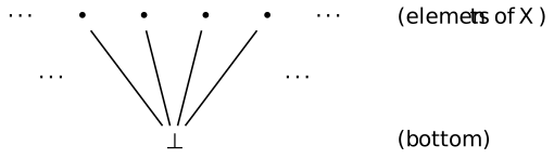
Formally, we say x \sqsubseteq y iff (x = y \lor x = \bot ).
Warning.
Don't confuse the information ordering on numbers, i.e. \sqsubseteq on \mathbb {Z}_\bot , with the numerical ordering \leq on \mathbb {Z}. We know 0 \leq 1, but 0 and 1 are not comparable in our flat information ordering.
Combining domains [dt-000D]
Some of our semantics may depend on the combination of multiple domains, i.e. semantic functions of multiple arguments. As an example, the semantics of an \mathsf {if} statement combines the semantics of the condition and the semantics of each of the two branches. In such scenarios, our domains are no longer flat — we must generalise to pointed posets.
DefinitionPointed poset [dt-000G]
A pointed poset is a partially ordered set with a bottom value.
ConstructionProduct of two pointed posets [dt-000E]
Given two pointed posets X and Y, the product poset X \times Y is ordered as follows: (x,y) \sqsubseteq _{X \times Y} (x',y') \quad \text {iff} \quad x \sqsubseteq _X x' \land y \sqsubseteq _Y y' Intuitively, this says that "the information content of a pair of values is increased by increasing the information of either or both of its component values".
This product poset is also pointed, with bottom value \bot _{X \times Y} being (\bot _A, \bot _B).
ExampleThe domain \mathbb {B}_\bot \times \mathbb {B}_\bot [dt-000F]
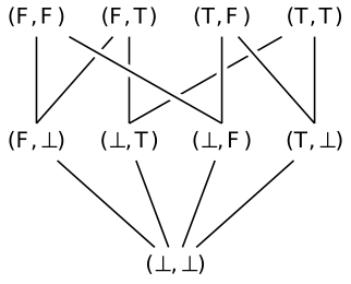
As can be seen above, the domain \mathbb {B}_\bot \times \mathbb {B}_\bot is not flat, but it is still a pointed poset.
Monotonic functions [dt-000H]
If we model our semantic domains for values with pointed posets, then programs are modelled by functions between such posets. But, not all functions are suitable:
ExampleThe halting query [dt-000I]
The function H : \mathbb {B}_\bot \rightarrow \mathbb {B}_\bot seems to let us solve the halting problem, assuming \bot represents non-termination: H(v) \; = \; \begin {cases} F & \text {if}\ v = \bot \\ T & \text {otherwise} \end {cases}
It stands to reason that the amount of information we get out of our functions should grow as we increase the amount of information we put into them. Such functions are called monotonic with respect to our information ordering.
DefinitionMonotonicity [dt-000J]
A function f : X \rightarrow Y between posets X and Y is monotone (or monotonic) if, for all x, y \in X: x \sqsubseteq y\; \text {implies}\; f(x) \sqsubseteq f(y)
DefinitionStrictness [dt-000K]
A function f : X \rightarrow Y on pointed posets X and Y is strict if it preserves the bottom value, i.e. f(\bot _X) = \bot _Y.
Thesis.
Computable functions are monotonic (observe that H is not).
Exercise [dt-000N]
Consider the functions \mathbb {B}_\bot \rightarrow \mathbb {B}_\bot . Which ones are monotonic? There are a total of 27 such functions but only three significant classes.
Solution.
Exercise [dt-000O]
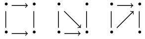
Let \mathbf {K}_K denote the chain of values x_1, x_2, x_3, \dots , x_K where a \leq b implies x_a \sqsubseteq x_b. There is one monotonic function \mathbf {K}_1 \rightarrow \mathbf {K}_1:

And there are three monotonic functions \mathbf {K}_2 \rightarrow \mathbf {K}_2:
- Write down the monotonic functions \mathbf {K}_3 \rightarrow \mathbf {K}_3.
- Write a simple recursive program to calculate the number of monotonic functions \mathbf {K}_n \rightarrow \mathbf {K}_m.
Solution.
When drawn as a diagram like the above, the monotonic functions are all those whose lines do not cross.
Solution.
In Haskell:
monotonics :: Int -> Int -> Int
monotonics n 1 = 1
monotonics n m = sum [monotonics (n-x) (m-1) | x <- [0..n]]
Fixed points [dt-000U]
From recursion to fixed points [dt-000R]
Consider our recursive \mathsf {while} loop semantics from § [dt-0006]: \llbracket \mathsf {while}\ b\ \mathsf {do}\ c\ \mathsf {od} \rrbracket _\mathcal {C}\ \sigma \; = \; \begin {cases} \llbracket \mathsf {while}\ b\ \mathsf {do}\ c\ \mathsf {od} \rrbracket _\mathcal {C}\ (\llbracket c \rrbracket _\mathcal {C}\ \sigma ) & \text {if}\ \llbracket b \rrbracket _\mathcal {B}\ \sigma = \mathit {T} \\ \sigma & \text {otherwise} \end {cases} How do we ensure that solutions exist for such recursive equations? And, if multiple solutions exist, how do we decide which one to pick? To address these questions, let's factor out everything in our definition except the recursion into a separate (higher-order) function: \begin {array}{l} \llbracket \mathsf {while}\ b\ \mathsf {do}\ c\ \mathsf {od} \rrbracket _\mathcal {C} = f(\llbracket \mathsf {while}\ b\ \mathsf {do}\ c\ \mathsf {od} \rrbracket _\mathcal {C}) \\[0.5em] \qquad \text {where}\; f(X)\ \sigma \; \triangleq \; \begin {cases} X\ (\llbracket c \rrbracket _\mathcal {C}\ \sigma ) & \text {if}\ \llbracket b \rrbracket _\mathcal {B}\ \sigma = \mathit {T} \\ \sigma & \text {otherwise} \end {cases} \end {array} Looking at it this way, we can see that any solution to this equation must be an element of our semantic domain X \in \mathbf {C} such that f(X) = X. In other words, the problem of finding solutions to our recursive equations can be cast as the problem of finding a fixed point for non-recursive higher-order functions.
DefinitionFixed point [dt-000S]
A value x is a fixed point of a function f if f(x) = x.
Monotonicity is insufficient [dt-000T]
Exercise [dt-000Q]
- Give an example of a poset A and a monotonic function f : A \rightarrow A such that f doesn't have a fixed point.
Solution.
In the poset (\mathbb {N},\leq ), the function f(x) = x + 1 has no fixed points.
- Give an example of a poset A and a monotonic function f : A \rightarrow A such that f has multiple fixed points.
Solution.
In the poset (\mathbb {N},\leq ), the function f(x) = x has infinitely many fixed points.
Problem.
Not all monotonic functions on posets have fixed points, and some have multiple fixed points!
So, requiring our functions to be monotonic is insufficient to guarantee that a single "best" solution exists.
Chains and Unfolding [dt-000Y]
- with contributions from Liam O'Connor
Intuitively, recursive programs are executed by "unfolding" as much as necessary to get a result. We would like to characterise our domains to ensure that solutions always exist, and to allow us to pick the solutions that are "minimal" in the sense that they rely on a minimal amount of unfolding.
After converting a recursive program into a non-recursive monotonic higher order function f, the fixed point we desire would intuitively be the limit of the ascending Kleene chain of f, i.e. f(f(f(f(\dots )))):
ExampleAscending Kleene chain [dt-000X]
Given a pointed poset (X,\subseteq ) and a monotonic function f : X \rightarrow X, the ascending Kleene chain is the \omega -chain: \bot \sqsubseteq f(\bot ) \sqsubseteq f(f(\bot )) \sqsubseteq f(f(f(\bot ))) \sqsubseteq \cdots Because \bot is the bottom element, we know that \bot \sqsubseteq f(\bot ). Each subsequent step in the chain exists because of monotonicity.
Each successive element of this chain is another "unfolding" of the recursion.
DefinitionChain [dt-000V]
A chain in a poset X is a totally ordered subset of X. That is, a subset Y \subseteq X is a chain iff: \forall x, y \in Y.\; x \sqsubseteq y \lor y \sqsubseteq x
Definition\omega -chain [dt-000W]
From chains to directed sets [dt-000Z]
- with contributions from Liam O'Connor
While \omega -chains are technically sufficient for denotational semantics, for our purposes it is a little more convenient to think in terms of directed sets rather than chains.
DefinitionDirected set [dt-0010]
Formally, a non-empty subset Y \subseteq X of a poset (X,\sqsubseteq ) is directed iff: \forall x, y \in Y.\ \exists z \in Y.\ x \sqsubseteq z \land y \sqsubseteq z
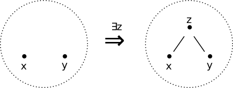
Intuitively, directed sets are "going somewhere" — given two elements we can always find a "greater" one in the set.
ExamplePower sets are directed [dt-0011]
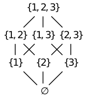
TheoremChain → Directed [dt-0012]
All non-empty chains are directed.
Proof.
Let C be a chain. Then, given two elements x,y \in C we know from totality that either x \sqsubseteq y or y \sqsubseteq x. If x \sqsubseteq y, then y is the upper bound, otherwise x is the upper bound.
DefinitionConsistent subset [dt-0013]
A subset Y \subseteq X of a poset X is consistent iff
\exists x \in X.\ \forall y \in Y.\ y \sqsubseteq x
Such an x is called an upper bound of Y.
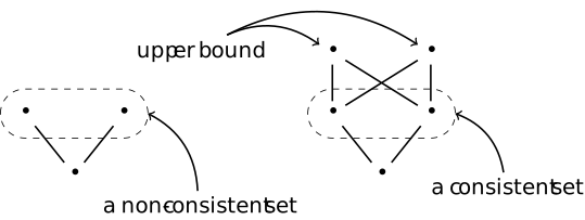
TheoremAlternative characterisation of directedness [dt-0014]
A subset Y \subseteq X of a poset X is directed iff every finite subset of Y' \subseteq Y has an upper bound in Y.
Proof.
- ⇐: Every pair of elements x,y \in Y has an upper bound simply by taking the upper bound of the set \{x,y\}.
- ⇒: Given a finite set X = \{x_1,x_2,\dots , x_n\} , we can show it has an upper bound by an inductive process, first taking the upper bound of x_1 and x_2, and then taking the upper bound of that an x_3 and so on until we have an upper bound for the whole set. This induction works because the set X is finite.
Corollary [dt-0015]
Least upper bounds [dt-0016]
DefinitionLeast upper bound [dt-0017]
Let X \subseteq Y be a subset of a poset Y. An element y \in Y is a least upper bound (or lub) for X iff:
- It is an upper bound: \forall x \in X.\ x \sqsubseteq y
- It is less than any other upper bound: \forall y' \in Y.\ (\forall x \in X. x \sqsubseteq y') \Rightarrow y \sqsubseteq y'
CorollaryProperties of \sqcup [dt-0018]
When lubs exist, the binary \sqcup operator is idempotent, commutative, and associative. Also, we have that x \sqsubseteq y iff x \sqcup y = y.
TheoremPointedness via lubs [dt-0019]
A poset Y is pointed iff \bigsqcup \emptyset exists, as the lub of an empty set is just the bottom element in the poset, i.e. \bigsqcup \emptyset = \bot .
Information intuition [dt-001A]
When the poset Y from Definition [dt-0017] is ordered by our information ordering, the intuition of the lub \bigsqcup X is that it combines all of the information content of all the elements of X but it does not add any additional information (hence least).
ExampleLubs in the domain \mathbb {B}_\bot \times \mathbb {B}_\bot [dt-001B]
- (\bot , \mathit {F}) \sqcup (\mathit {T},\bot ) = (\mathit {T},\mathit {F})
- (\bot , \mathit {F}) \sqcup (\bot ,\bot ) = (\bot ,\mathit {F})
- (\bot , \mathit {F}) \sqcup (\mathit {T}, \mathit {T}) does not exist.
Exercise [dt-001C]
Complete partial orders [dt-001E]
DefinitionComplete partial order [dt-001D]
A complete partial order or cpo (more specifically a directed complete partial order or dcpo) is a poset where lubs exist for the empty set and for all directed subsets. That is, a cpo is a poset A such that:
- A has a bottom element \bot \in A, that is the lub of the empty set, and
- \bigsqcup X exists for all directed X \subseteq A.
AsideOther kinds of completeness [dt-001F]
In Definition [dt-001D] we defined cpos in terms of directed completeness. We may consider chain completeness instead, where, rather than require lubs for every directed subset of our poset A, we require lubs for every chain X \subseteq A. We know from Theorem [dt-0012] that all chains are directed, so every directed complete cpo is also chain complete. It is also known that every chain complete cpo is also directed complete, so the notions are equivalent, although the proof is non-trivial, relying on transfinite induction (see these lecture notes for details).
If we weaken our completeness requirement to require lubs only for the countable \omega -chains and not necessarily all chains, we get what is called an \omega -cpo. All \omega -chains are chains and are therefore directed, but not all chains are \omega -chains.
Working with just \omega -cpos is common in denotational semantics practice, but working with directed completeness simplifies some of the properties we will discuss later.
Exercise [dt-001G]
For each of the following posets, determine if it is a cpo or not. If it is, describe the lubs. If it is not, give a directed set which has no lub.
- A finite pointed poset
- (\mathcal {P}(S), \subseteq ) for some set S
- (\mathbb {N},\leq )
- (\mathbb {N} \cup \{\infty \}, \leq )
- ([0,1] \subseteq \mathbb {R}, \leq )
- ([0,1) \subseteq \mathbb {R}, \leq )
- (\mathbb {Q}, \leq )
- A flat domain S_\bot for some set S.
Solution.
- A finite pointed poset is a cpo, as all directed subsets will be finite and therefore have a lub.
- (\mathcal {P}(S), \subseteq ) is a cpo as the lub is just the union.
- (\mathbb {N},\leq ) is not a cpo, as the \omega -chain 1 \leq 2 \leq 3 \leq \cdots has no lub.
- (\mathbb {N} \cup \{\infty \}, \leq ) is a cpo, as \infty is the lub of any non-repeating chain.
- ([0,1] \subseteq \mathbb {R}, \leq ) is a cpo with maximum as the lub.
- ([0,1) \subseteq \mathbb {R}, \leq ) is not a cpo, as the set \{0.9,0.99,0.999,\dots \} has a lub of 1 \notin [0,1).
- (\mathbb {Q}, \leq ) is not a cpo, and not just because it lacks a lub for \mathbb {Q} itself, but also it doesn't contain \sqrt {2}, which can be expressed as the lub of an infinite sequence of rational approximations.
- A flat domain S_\bot for some set S is a cpo, as the largest chains have two elements, and we always pick the non-\bot one as the lub.
RemarkLubs of chains [dt-001H]
The limit of the ascending Kleene chain of a monotonic function f : X \rightarrow X is the same as the least upper bound of the set \{ f^n(\bot ) \mid n \in \mathbb {N}\} (where f^n is the n-fold self-composition of the function f). If we require that our semantic domain X is a cpo, we know that this limit exists.
Our semantic domains are cpos, ensuring the presence of these limits.Thesis.
Exercise [dt-001X]
- Show that if A and B are posets and X \subseteq A \times B is directed (by the ordering in Construction [dt-000E]), then the subsets \pi _0(X) \subseteq A and \pi _1(X) \subseteq B (defined below) are also directed.
\begin {array}{lcl}
\pi _0(X) & = & \{ a \in A \mid \exists b \in B.\ (a,b) \in X \}\\
\pi _1(X) & = & \{ b \in B \mid \exists a \in A.\ (a,b) \in X \}\\
\end {array}
Solution.
Given two elements x,y \in \pi _0(X), we know that there exists b_x, b_y \in B such that (x,b_x) \in X and (y,b_y) \in X. Because X is directed, we can conclude that there exists an upper bound (z, b_z) \in X where x \sqsubseteq z and y \sqsubseteq z. As z \in \pi _0(X), z is an upper bound in \pi _0(X) for both x and y and thus \pi _0(X) is directed. The proof for \pi _1 is analogous.
- Give an example of a set X \subseteq \{\top ,\bot \}\times \{\top ,\bot \} such that \pi _0(X) and \pi _1(X) are directed, but X is not.
Solution.
X = \{(\top ,\bot ), (\bot ,\top )\} is not directed as the two elements are not comparable, but \pi _0(X) = \pi _1(X) = \{\top ,\bot \} which is directed as \bot \sqsubseteq \top .
- Show that if A and B are cpos and X \subseteq A \times B is directed, then \bigsqcup X = \left (\bigsqcup \pi _0(X), \bigsqcup \pi _1(X)\right ) Note: Together with \bot _{A\times B} = (\bot _A, \bot _B) this shows that the Cartesian product of two cpos is itself a cpo.
Solution.
Let (x,y) = \left (\bigsqcup \pi _0(X), \bigsqcup \pi _1(X)\right ). Because of the ordering in Construction [dt-000E], (x,y) is certainly a upper bound of the directed set X. To show it is the least upper bound, assume for the sake of contradiction that (x,y) is not the least upper bound of X. Then, there must be a (v,w)\sqsubset (x,y) such that \forall x \in X.\ x \sqsubseteq (v,w). But then, v would be a lesser upper bound for \pi _0(X) than x, which is supposed to be the lub. Thus there is a contradiction, and (x,y) must be the lub of X.
Continuity and Fixed Points [dt-001I]
- with contributions from Liam O'Connor
By choosing a cpo for our semantic domain, we can ensure that the Kleene chain has a limit. However, it is not guaranteed that the limit we find will be a fixed point to our monotonic function f.
ProblemMonotonicity is insufficient [dt-001K]
Consider this monotonic function g defined over a cpo (\mathbb {R} \cup \{\infty ,-\infty \}, \leq ): g(x) = \begin {cases} \tan ^{-1} x & \text {if}\ x < 0\\ 1 & \text {otherwise} \end {cases} Note this function is not continuous at 0. Starting from our \bot element -\infty , we can see that the limit of the ascending Kleene chain is 0: \begin {array}{lcl} g(-\infty ) & = & -\frac {\pi }{2}\\ g(-\frac {\pi }{2}) & = & -1\\ g(-1) & \approx & -0.78\\ \end {array} But g(0) = 1! — the lub of the Kleene chain is not a fixed point!
To address this problem, we shall strengthen our requirement on functions from mere monotonicity to continuity.
DefinitionContinuity [dt-001J]
A function f : A \rightarrow B on cpos A and B is continuous iff for all directed X \subseteq A,
- \bigsqcup \{ f(x) \mid x \in X \} exists, and
- f(\bigsqcup X) = \bigsqcup \{ f(x) \mid x \in X \}, i.e., f preserves lubs.
TheoremContinuity implies monotonicity [dt-001L]
All continuous functions are monotonic.
Consider two elements x, y of a cpo where x \sqsubseteq y. Then \{x,y\} is directed with a lub of y. By the second condition in Definition [dt-001J], we get f(y) = f(x) \sqcup f(y) which is equivalent to f(x) \sqsubseteq f(y).Proof.
ExampleMonotonic but not continuous [dt-001M]
Consider this function from \mathbb {N} \cup \{\infty \} \rightarrow \{\top ,\bot \}, defined by: f(x) = \begin {cases} \bot & \text {if}\ x \in \mathbb {N}\\ \top & \text {otherwise} \end {cases} This function is monotonic, but, taking X = \mathbb {N} (which is a directed subset of the cpo \mathbb {N} \cup \{\infty \}), then f(\bigsqcup \mathbb {N}) = f(\infty ) = \top , but \bigsqcup \{ f(n) \mid n \in \mathbb {N} \} = \bigsqcup \{ \bot \} = \bot . Thus, this function is not continuous.
Exercise [dt-001N]
Show that if a function on cpos f : A \rightarrow B is monotonic, then \bigsqcup \{ f(x) \mid x \in X \} exists for any directed X \subseteq A (i.e.the first condition for continuity in Definition [dt-001J]).
Hint: It suffices to show that \{ f(x) \mid x \in X \} \subseteq B is directed.
Solution.
Because B is a cpo, it suffices to show that \{ f(x) \mid x \in X \} \subseteq B is directed. Let a,b \in \{ f(x) \mid x \in X \}. Let x_a, x_b \in X be the values that f maps to a and b respectively, i.e. f(x_a) = a and f(x_b) = b. Because X is directed, an upper bound of x_a and x_b exists in X. Call this upper bound x_c. Because x_a \sqsubseteq x_c and x_b \sqsubseteq x_c, we know that f(x_a) = a \sqsubseteq f(x_c) and f(x_b) = b \sqsubseteq f(x_c) by monotonicity of f. Also, f(x_c) \in \{ f(x) \mid x \in X \} because x_c \in X. Therefore, because two arbitrary elements in \{ f(x) \mid x \in X \} have an upper bound within the set, the set \{ f(x) \mid x \in X \} is directed.
TheoremAlternative characterisation of continuity [dt-001O]
A function f : A \rightarrow B on cpos A and B is continuous iff:
- f is monotonic, and
- f(\bigsqcup X) = \bigsqcup \{ f(x) \mid x \in X \}, for all directed X \subseteq A
Proof.
The second condition here is identical to that of Definition [dt-001J]. The monotonicity requirement is equivalent to the first condition of Definition [dt-001J], with one direction shown by Theorem [dt-001L], and the other shown by the solution of Exercise [dt-001N].
Thesis.
Computable functions are continuous functions on cpos.
Exercise [dt-001W]
Show that if a function f : A \rightarrow B on cpos A and B is monotonic and A is finite, then f is continuous.
Hint: Finite directed sets contain their lub
Solution.
Because of Theorem [dt-001O], it suffices to show the second condition of continuity, as f is monotonic.
Because A is finite, any directed subset X \subseteq A is also finite, and therefore \bigsqcup X \in X. Because f is monotone, f(x) \sqsubseteq f (\bigsqcup X) for all x \in X.
The solution to Exercise [dt-001N] shows that \{f(x) \mid x \in X\} is directed and therefore contains its upper bound c. Because f is monotone, f(\bigsqcup X) must be c (else it would contradict the above).
Therefore \bigsqcup \{f(x) \mid x \in X\} = f (\bigsqcup X), as required.
TheoremThe Kleene fixed point theorem [dt-001P]
Let (S, \sqsubseteq ) be a cpo and f : S \rightarrow S be a continuous function. Then the lub of the Kleene chain \bigsqcup _{n\in \mathbb {N}}f^{n}(\bot ) is the least fixed point of f.
Proof.
We apply continuity to show that it is a fixed point: \begin {array}{lclr} f(\bigsqcup _{n \in \mathbb {N}} f^n(\bot ) ) & = & \bigsqcup _{n \in \mathbb {N}} f(f^n(\bot )) & \text {(continuity)} \\[0.5em] &=& \bigsqcup _{n \in \mathbb {N}} f^{n+1}(\bot )\\[0.5em] &=& \bigsqcup _{n=1,2\dots }f^{n}(\bot ) &\qquad \text {(reindexing)}\\[0.5em] &=& \bot \sqcup \bigsqcup _{n=1,2\dots }f^{n}(\bot )\\[0.5em] &=&\bigsqcup _{n\in \mathbb {N}}f^{n}(\bot )\\[0.5em] \end {array} To see that it is the least fixed point: Let y be a fixed point of f. We know that \bot \sqsubseteq y by definition of \bot . Taking f of both sides, we get f(\bot ) \sqsubseteq y. We can continue this inductively and thus we know that, for all n \in \mathbb {N}, f^n(\bot ) \sqsubseteq y. Because y is, therefore, an upper bound of the ascending Kleene chain, it must also be at least as large as the lub of that chain.
DefinitionThe \textbf {fix} operator [dt-001Q]
Let \textbf {fix}(f) denote the least fixed point of the continuous function f, that is \bigsqcup _{n\in \mathbb {N}}f^{n}(\bot ), guaranteed to exist by Theorem [dt-001P].
Exercise [dt-001S]
- What is \textbf {fix}(\mathsf {id}) where \mathsf {id} is the identity function on \mathbb {B}_\bot ?
Solution.
\bigsqcup \{ \bot , \mathsf {id}(\bot ), \mathsf {id}(\mathsf {id}(\bot )), \dots \} = \bot - What is \textbf {fix}(\kappa _\mathit {F}) where \kappa _\mathit {F} is the constant function that always returns \mathit {F}?
Solution.
\bigsqcup \{ \bot , \kappa _F(\bot ), \kappa _F(\kappa _F(\bot )), \dots \} = \mathit {F} - What is \textbf {fix}(f) where
\begin {array}{l}
f : [\mathbb {N}_\bot ] \rightarrow [\mathbb {N}_\bot ]\\
f(x) = 1::x
\end {array}
(where [\mathbb {N}_\bot ] denotes Haskell-style lazy lists of \mathbb {N}_\bot )?
Solution.
\bigsqcup \{ \bot , 1::\bot , 1::1::\bot , \dots \} = 1::1::1::\cdots Here \textbf {fix}(f) would be the semantics of the recursive definition \mathsf {ones} = 1 :: \mathsf {ones}.
Semantics with fixed points [dt-001R]
Semantics of loops [dt-001V]
Armed with the \textbf {fix} operator, we can return to our semantics of \mathsf {while} loops from § [dt-0006] and § [dt-000R], and at last define their semantics without relying on dubious recursive definitions: \begin {array}{l} \llbracket \mathsf {while}\ b\ \mathsf {do}\ c\ \mathsf {od} \rrbracket _\mathcal {C} = \textbf {fix}(f)\\[0.5em] \qquad \text {where}\; f(X)\ \sigma \; \triangleq \; \begin {cases} X\ (\llbracket c \rrbracket _\mathcal {C}\ \sigma ) & \text {if}\ \llbracket b \rrbracket _\mathcal {B}\ \sigma = \mathit {T} \\ \sigma & \text {otherwise} \end {cases} \end {array}
Proof that f is continuous is technically required but is omitted here.
ExampleSemantics of recursive functions [dt-001U]
Consider the function \Phi \in (\mathbb {N}_\bot \rightarrow \mathbb {N}_\bot ) \rightarrow (\mathbb {N}_\bot \rightarrow \mathbb {N}_\bot ), given by: \Phi (f) = \lambda n.\ \text {if}\ n = 0\ \text {then}\ 1\ \text {else}\ n\cdot f(n-1) Looking at the first few elements of our Kleene chain, we get: \begin {array}{lcl} \Phi ^0(\bot ) & = & \lambda n.\ \bot \quad \text {(i.e. $\bot _{\mathbb {N}_\bot \rightarrow \mathbb {N}_\bot }$)}\\ \Phi ^1(\bot ) & = & \lambda n.\ \text {if}\ n = 0\ \text {then}\ 1\ \text {else}\ \bot \\ \Phi ^2(\bot ) & = & \lambda n.\ \text {if}\ n = 0\ \text {then}\ 1\ \text {else}\ n\cdot (\text {if}\ n - 1 = 0\ \text {then}\ 1\ \text {else}\ \bot )\\ \cdots \end {array} Continuing on, we see that the mth approximation \Phi ^m(\bot ) to \textbf {fix}(\Phi ) is the function that gives x! for all x up to m, and diverges (\bot ) for all other arguments. Hence the limit \textbf {fix}(\Phi ) is the factorial function on \mathbb {N}_\bot !
Exercise [dt-001T]
- Write down the first few approximations \Phi ^m(\bot ) to \textbf {fix}(\Phi ), where the higher order function \Phi : (\mathbb {Z}_\bot \rightarrow [\mathbb {Z}_\bot ]) \rightarrow (\mathbb {Z}_\bot \rightarrow [\mathbb {Z}_\bot ]) is given by: \Phi (f) = \lambda n.\ n :: f (n+1) What is \Phi ^m(\bot )? What is \textbf {fix}(\Phi )?
- Repeat the same process, but this time for a new higher order function \Phi : (\mathbb {Z}_\bot \rightarrow \mathbb {Z}_\bot ) \rightarrow (\mathbb {Z}_\bot \rightarrow \mathbb {Z}_\bot ) given by: \Phi (f) = \lambda n.\ \text {if}\ n = 0\ \text {then}\ 0\ \text {else}\ f(n-2)
Solution.
The approximations are \{ \lambda n.\ \bot , \lambda n.\ n :: \bot , \lambda n.\ n :: (n + 1) :: \bot , \dots \}. The limit is a function that, given a natural number n, produces the infinite list of natural numbers starting from n.
Solution.
The nth approximation returns 0 if the input number is non-negative, even and less than 2n, otherwise it diverges (returns \bot ). The limit returns 0 for any non-negative even number, and diverges otherwise.