Lecture. Domain theory › Constructions on cpos and PCF [dt-001Z]
This lecture is based on material from Graham Hutton, John Longley, Dana Scott, Joseph Stoy, Carl Gunter, and Glynn Winskel.
Products [dt-002K]
Recall Construction [dt-000E], which showed that the product of two pointed posets is itself a pointed poset. In Exercise [dt-001X] you may also have shown that A \times B is also a cpo if A and B are cpos, with this definition for lubs: \bigsqcup X \; = \; \left (\bigsqcup \{ x \mid \exists y.\ (x,y) \in X \}, \bigsqcup \{ y \mid \exists x.\ (x,y) \in X \}\right ) This definition can be made a little more comprehensible by defining it in terms of the two projection operators for pairs:
DefinitionProjection operators for products [dt-0020]
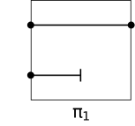
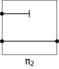
Destruction of pairs is captured by the two projection operators, defined as follows:
|
\begin {array}{lcl} \pi _0 : A \times B \rightarrow A & \qquad & \pi _1 : A \times B \rightarrow B \\ \pi _0(x, y) = x & & \pi _1(x, y) = y \\ \end {array} |
|
ConstructionProduct of cpos [dt-0021]
Given cpos A and B, the product A \times B is itself a cpo, ordered by (x,y) \sqsubseteq _{X \times Y} (x',y') \quad \text {iff} \quad x \sqsubseteq _X x' \land y \sqsubseteq _Y y' with bottom value \bot _{X \times Y} being (\bot _A, \bot _B). Least upper bounds are found by taking the lubs of each component:
\bigsqcup X \; = \; \left (\bigsqcup \{ \pi _0(x) \mid x \in X \}, \bigsqcup \{ \pi _1(x) \mid x \in X \}\right )TheoremContinuity of projection operations [dt-0022]
The projection functions \pi _0 and \pi _1 are continuous.
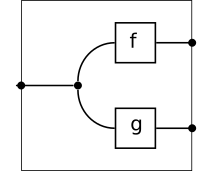
DefinitionThe split function [dt-0023]
TheoremContinuity of split [dt-0024]
For continuous functions f and g, the split function \langle f, g \rangle is continuous.
Proof.
Using the alternative characterisation of continuity:
- \langle f, g \rangle is monotonic. Let x \sqsubseteq y \in A. Then: \begin {array}{lclr} \langle f , g \rangle \ x & = & (f(x), g(x)) & \text {(def)}\\ & \sqsubseteq & (f(y), g(y)) & \text {(monotonicity of $f$,$g$)}\\ & = & \langle f , g \rangle \ y & \text {(def)} \end {array}
- \langle f , g \rangle preserves lubs of directed sets. Let X \subseteq A be directed. Then: \begin {array}{lclr} \langle f , g \rangle \ (\bigsqcup X) & = & (f(\bigsqcup X), g(\bigsqcup X)) & \text {(def)}\\ & = & (\bigsqcup \{ f(x) \mid x \in X \}, \bigsqcup \{ g(x) \mid x \in X \}) & \text {(continuity of $f$,$g$)}\\ & = & \bigsqcup \{ \langle f , g \rangle \ x \mid x \in X \} & \text {(def)} \end {array}
These building blocks can be used to make many functions on products (thereby ensuring continuity):
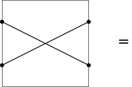
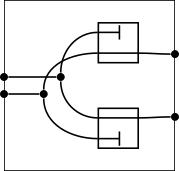
DefinitionThe \mathit {swap} function [dt-0025]
 |
|
\begin {array}{l}\mathit {swap} : A \times B \rightarrow B \times A \\ \mathit {swap} = \langle \pi _1 , \pi _0 \rangle \end {array} |
DefinitionProduct of functions [dt-0026]
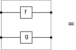
Given f : A \rightarrow C and g : B \rightarrow D, we overload the \times operator for products to denote the combined function f \times g : A \times B \rightarrow C \times D, given below:
 |
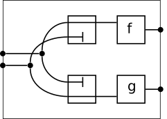 |
\begin {array}{l} f \times g : A \times B \rightarrow C \times D \\ f \times g = \langle f \circ \pi _0 , g \circ \pi _1 \rangle \end {array} |
Exercise [dt-002G]
Express the function \mathit {juggle} (a, (b,c)) = ((a,b),c) using just our primitive combinators for projection and split.
Solution.
\mathit {juggle} \triangleq \langle \langle \pi _0 , \pi _0 \circ \pi _1 \rangle , \pi _1 \circ \pi _1 \rangle
Pictorial Properties [dt-0027]
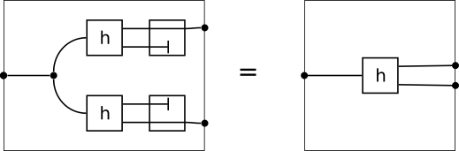
The following properties of our projection and split functions follow from the pictorial reasoning we see on the right:
| \pi _0 \circ \langle f , g \rangle = f | 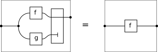 |
| \pi _1 \circ \langle f , g \rangle = g | 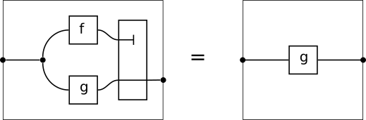 |
| \langle \pi _0 \circ h , \pi _1 \circ h \rangle = h |
 |
Exercise [dt-0028]
Prove that the three properties in § [dt-0027] are equivalent to the universal property for products
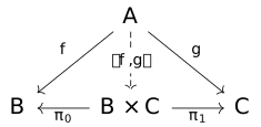
(\pi _0 \circ h = f \land \pi _1 \circ h = g)\ \text {iff}\ h = \langle f , g \rangleSolution.
Showing in both directions:
- The three properties follow from the universal property: The first two properties follow from the universal property where h is set to \langle f , g \rangle . The third property follows from the universal property where f is set to \pi _0\circ h and g is set to \pi _1\circ h.
- The universal property follows from the universal property: In the \Rightarrow direction of the universal property follows from the third property, and the \Leftarrow direction follows from the first two.
DefinitionUniversal property for cpo products [dt-0029]
As commuting diagram on the category \mathbf {Cpo}:
AsideCategory theory [dt-002A]
DefinitionCategory [dm-000G]
A category Cconsists of a collection of things (objects) and a collection of arrows between these things (morphisms). If there is a morphism A \xrightarrow {f} B and a morphism B \xrightarrow {g} C, we also have the composed morphism A \xrightarrow {g \circ f} C. This composition operator must be associative. Additionally each object X has an identity morphism X \xrightarrow {\mathsf {id}_X} X, such that for an arrow X \xrightarrow {a} Y, a \circ \mathsf {id}_X = \mathsf {id}_Y \circ a = a.
ExampleThe category \mathbf {Set} [dm-000H]
ExampleThe category \mathbf {Rel} [dm-000I]
ExampleThe category \mathbf {Cpo} [dt-002B]
The category \mathbf {Cpo} is the category where the objects are cpos, the morphisms are continuous functions between these cpos, composition is function composition ((g \circ f)(x) \triangleq g(f(x))) and identity is just the identity function \lambda x. x.
DefinitionFunctor [dm-000J]
A functor F from a category \mathbf {C} to a category \mathbf {D} consists of an object mapping that maps objects of \mathbf {C} to objects of \mathbf {D}, and a morphism mapping that maps morphisms of \mathbf {C} to morphisms of \mathbf {D} such that:
- For each A \xrightarrow {m} B in \mathbf {C}, we have a morphism F(A) \xrightarrow {F(m)} F(B) in \mathbf {D}.
- For each object A in \mathbf {C}, the equation F(\mathsf {id}_A) = \mathsf {id}_{F(A)} holds in \mathbf {D}.
- For a pair of morphism A \xrightarrow {f} B \xrightarrow {g} C in \mathbf {C}, the equation F (g \circ f) = F(g) \circ F(f) holds in \mathbf {D}.
ExampleThe category \mathbf {Cat} [dm-000K]
The category \mathbf {Cat} is the category where the objects are themselves (small) categories, the morphisms are structure-preserving maps between these categories, i.e., functors.
Commutative diagrams [dm-000L]
When working in a category, we can state many theorems compactly using commutative diagrams, such as this diagram for products:
CorollaryDerived properties of cpo products [dt-002C]
The universal property is called such because all the familiar properties of products follow from it – thinking in pictures helps to see how (Indeed, the universal property characterises products up to isomorphism):
- \pi _0 \circ (f \times g) = f \circ \pi _0
- \pi _1 \circ (f \times g) = g \circ \pi _1
- (f \times g) \circ \langle h , i \rangle = \langle f \circ h, g \circ i \rangle
- \langle f , g \rangle \circ h = \langle f \circ h, g \circ h \rangle
- \mathsf {id}_A \times \mathsf {id}_B = \mathsf {id}_{A \times B} \quad (*)
- (f \circ g) \times (h \circ i) = (f \times h) \circ (g \times i) \quad (**)
These last two statements (*) and (**) show that \times is a bifunctor on the category \textbf {Cpo}, i.e., a functor \textbf {Cpo} \times \textbf {Cpo} \rightarrow \textbf {Cpo}.
Exercise [dt-002I]
Show using the universal property that \langle f, g \rangle \circ h = \langle f \circ h , g \circ h \rangle
Solution.
Isomorphisms for cpo products [dt-002D]
DefinitionCpo isomorphism [dt-002E]
An isomorphism between two cpos A and B is a bijection f between A and B such that f preserves the cpo structure, i.e., that f and f^{-1} are continuous.
We say two cpos A and B are isomorphic, written A \simeq B, iff an isomorphism exists between them.
TheoremCommutative monoid structure for cpos [dt-002H]
Cpos form a commutative monoid "up to isomorphism" under \times and \mathbf {1} (the cpo consisting of only one element \bot ). That is, for all cpos A, B and C:
- A \times \mathbf {1} \simeq A
- A \times (B \times C) \simeq (A \times B) \times C
- A \times B \simeq B \times A
Proof.
The isomorphisms required are the projection \pi _0, the \mathit {juggle} function from Exercise [dt-002G], and the swap function.
DefinitionThe set of continuous functions [dt-002F]
Let A \twoheadrightarrow B denote just the continuous functions from cpo A to cpo B: A \twoheadrightarrow B\; \triangleq \; \{ f : A \rightarrow B \mid f\ \text {is continuous} \}
Theorem [dt-002J]
There is an isomorphism between pairs of continuous functions and continuous functions that output pairs: (A \twoheadrightarrow B) \times (A \twoheadrightarrow C)\; \simeq \; (A \twoheadrightarrow (B \times C))
Proof.
Upshot.
Because we have the functor \times on \textbf {Cpo} that satisfies the properties of products described above, the category \textbf {Cpo} therefore has binary products.
Functions [dt-002Z]
Previously, such as in Example [dt-001U], we already implicitly assumed that the set of continuous functions on cpos A \twoheadrightarrow B is itself a cpo. In this section, we will formalise this construction.
ConstructionThe cpo of functions [dt-002L]
If A and B are cpos, the set of continuous functions A \twoheadrightarrow B is a cpo under the pointwise ordering: f \sqsubseteq g\;\; \text {iff}\;\; \forall a \in A.\ f(a) \sqsubseteq g(a) The intuition of this ordering in terms of information is that we increase the information content of a function overall by increasing the information content of any (or many) argument values. To prove this, we must show:
- A \twoheadrightarrow B has a least element. \bot _{A \twoheadrightarrow B} is the constant function that returns \bot _B, i.e. \lambda a.\ \bot _B.
- \bigsqcup X exists for all directed X \subseteq A \twoheadrightarrow B. Our lub of a set of continuous functions \bigsqcup X is the function \Phi where: \Phi (a) = \bigsqcup \{ f(a) \mid f \in X\}
We must show a number of properties of this lub \Phi . Specifically:
- \bigsqcup \{ f(a) \mid f \in X\} exists in B.
Proof.
We want to show that the set \{ f(a) \mid f \in X\} is directed. Take two values g(a), h(a) \in \{ f(a) \mid f \in X\}. Since X is directed, there exists a function k \in X such that g \sqsubseteq k and h \sqsubseteq k. By applying the definition of \sqsubseteq for functions above, we have g(a) \sqsubseteq k(a) and h(a) \sqsubseteq k(a). Thus k(a) is an upper bound of these two values g(a), h(a), and thus \{ f(a) \mid f \in X\} is directed, and thus its lub exists since B is a cpo. - \Phi (a) = \bigsqcup \{ f(a) \mid f \in X \} is continuous.
Proof.
Using the alternative characterisation of continuity
\begin {array}{lclr} \Phi (\bigsqcup Y) &=& \bigsqcup \{ f(\bigsqcup Y) \mid f \in X \} & \text {(defn. $\Phi $)}\\ & = & \bigsqcup \{\bigsqcup \{ f(y) \mid y \in Y \} \mid f \in X \} & \text {($f$ is continuous)}\\ & = & \bigsqcup \{\bigsqcup \{ f(y) \mid f \in X \} \mid y \in Y \} & \text {(swap lubs)}\\ & = & \bigsqcup \{ \Phi (y) \mid y \in Y \} & \text {(defn. $\Phi $)}\\ \end {array} Monotonicity is similar to prove. - \Phi is an upper bound for X \subseteq A \twoheadrightarrow B.
Proof.
Let g \in X. Then for any a \in A we have g(a) \in \{ f(a) \mid f \in X\}. Now, by 2a and lubs, we have g(a) \sqsubseteq \bigsqcup \{ f(a) \mid f \in X \}, which by the definition of \Phi gives g(a) \sqsubseteq \Phi (a). Hence, by the definition of \sqsubseteq on functions, we can conclude g \sqsubseteq \Phi . - \Phi is the least upper bound for X.
Proof.
Let g \in A \twoheadrightarrow B be an upper bound for X \subseteq A \twoheadrightarrow B. Then (using \sqsubseteq on functions) g(a) is an upper bound for \{f(a) \mid f \in X\} for all a \in A. Now, by 2a and lubs, we have \bigsqcup \{f(a) \mid f \in X\} \sqsubseteq g(a), i.e. \Phi (a) \sqsubseteq g(a), which, by the definition of \sqsubseteq on functions, allows us to conclude \Phi \sqsubseteq g.
- \bigsqcup \{ f(a) \mid f \in X\} exists in B.
ExampleThe space \mathbb {B}_\bot \twoheadrightarrow \mathbb {B}_\bot [dt-002M]
 At each step "upwards" on this
Primitive functions for functions [dt-002P]
DefinitionThe \mathit {apply} function [dt-002N]
The \mathit {apply} function simply applies a given function to a given argument: \begin {array}{l} \mathit {apply} : ((A \twoheadrightarrow B) \times A) \twoheadrightarrow B\\ \mathit {apply} (f, a) = f(a) \end {array}
Exercise [dt-002Q]
Show that \mathit {apply} is continuous.
Hint: A function f : A \times B \rightarrow C is continuous iff it is continuous in each argument separately, i.e., iff \forall a \in A.\ f(a,\cdot ) : B \rightarrow C is continuous, and \forall b \in B.\ f(\cdot ,b) : A \rightarrow C is continuous.
Solution.
First showing \mathit {apply}(f,\cdot ) is continuous for some continuous f : A \twoheadrightarrow B, using the alternative characterisation
- \mathit {apply}(f,\cdot ) is monotonic: Given a, b \in A where a \sqsubseteq b, we can see that \mathit {apply}(f,a) = f(a) \sqsubseteq f(b) = \mathit {apply}(f,b) by the monotonicity of f.
- \mathit {apply}(f,\cdot ) preserves lubs: Given a directed X \subseteq A, we can see that \mathit {apply}(f,\bigsqcup X) = f(\bigsqcup X) = \bigsqcup \{f(x) \mid x \in X\} = \bigsqcup \{\mathit {apply}(f,x) \mid x \in X\} follows from the continuity of f.
- \mathit {apply}(\cdot ,a) is monotonic: Given f, g \in A \twoheadrightarrow B where f \sqsubseteq g, we can see that \mathit {apply}(f,a) = f(a) \sqsubseteq g(a) = \mathit {apply}(g,a) by the pointwise ordering of functions.
- \mathit {apply}(\cdot ,a) preserves lubs: Given a directed X \subseteq A \twoheadrightarrow B, we can see that \mathit {apply}(\bigsqcup X, a) = \left (\bigsqcup X\right )(a) = \bigsqcup \{f(a) \mid f \in X\} = \bigsqcup \{\mathit {apply}(f,a) \mid f \in X\} follows from the lub definition for functions.
DefinitionThe \mathit {curry} function [dt-002O]
The function \mathit {curry} transforms a function that takes two arguments all at once (as a product) into a function that takes the arguments one at a time. That is, if f : A \times B \twoheadrightarrow C then: \begin {array}{l} \mathit {curry}(f) : A \twoheadrightarrow (B \twoheadrightarrow C)\\ \mathit {curry}(f)(a)(b) = f(a, b) \end {array}
TheoremContinuity of \mathit {curry} [dt-002S]
- \mathit {curry} is continuous on A \times B \twoheadrightarrow C.
- \mathit {curry}(f), given continuous f : A \times B \twoheadrightarrow C, is continuous on A.
- \mathit {curry}(f)(a), given continuous f : A \times B \twoheadrightarrow C and a \in A, is continuous on B.
Exercise [dt-002R]
What is the common (functional programming) name for \mathit {apply} \circ (f \times \mathsf {id})?
\mathit {uncurry}Solution.
DefinitionUniversal property for functions [dt-002T]
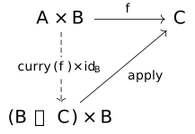
TheoremThe currying isomorphism [dt-002U]
Proof.
Follows from the universal property for functions when set up with the isomorphism from curry and its inverse, the function in Exercise [dt-002R].
RemarkWhy the function arrow is not a covariant bifunctor [dt-002V]
For the \twoheadrightarrow operator on cpos (Definition [dt-002F]) to be the object mapping for a bifunctor \textbf {Cpo} \times \textbf {Cpo} \rightarrow \textbf {Cpo} like \times is (see Corollary [dt-002C]), we would need to define a morphism mapping f \twoheadrightarrow g that, given two functions f : A \twoheadrightarrow B and g : C \twoheadrightarrow D, gives a function (A \twoheadrightarrow C) \twoheadrightarrow (B \twoheadrightarrow D). But such a function is not implementable: \begin {array}{l} f \twoheadrightarrow g : (A \twoheadrightarrow C) \twoheadrightarrow (B \twoheadrightarrow D) \\ (f \twoheadrightarrow g)(h)(b) =\ \textcolor {red}{???}\\ \end {array} In the above hole \textcolor {red}{???}, h : A \twoheadrightarrow C and b \in B. Given the value b \in B, none of our functions f, g or h take elements of B, so there would be no way to produce the D value required. This is because our function f : A \twoheadrightarrow B goes the wrong way. If f were a function B \twoheadrightarrow A, things would be a lot easier.
DefinitionDual category [dm-000Q]
The function arrow is a bifunctor [dt-002W]
The operator \twoheadrightarrow introduced in Definition [dt-002F] is is the object mapping for a binary functor: (\twoheadrightarrow ) : \mathbf {Cpo}^\mathsf {op} \times \mathbf {Cpo} \rightarrow \mathbf {Cpo} The category \mathbf {Cpo}^\mathsf {op} is the dual category to \mathbf {Cpo}.
Thus, a morphism A \xrightarrow {m} B in the category \mathbf {Cpo}^\mathsf {op} is a continuous function m : B \twoheadrightarrow A. Thus, the morphism mapping for our functor must take two functions f : B \twoheadrightarrow A (the morphism from \mathbf {Cpo}^\mathsf {op}) and g : C \twoheadrightarrow D (the morphism from \mathbf {Cpo}), and produce (A \twoheadrightarrow C) \twoheadrightarrow (B \twoheadrightarrow D). As with products, we will overload the \twoheadrightarrow notation for this mapping as well.
DefinitionMorphism mapping for \twoheadrightarrow [dt-002X]
Given f : B \twoheadrightarrow A and g : C \twoheadrightarrow D, we have: \begin {array}{l} f \twoheadrightarrow g : (A \twoheadrightarrow C) \twoheadrightarrow (B \twoheadrightarrow D)\\ f \twoheadrightarrow g = \mathit {curry}\ (g \circ \mathit {apply} \circ (\mathsf {id} \times f))\\[2em] \text {(or, operationally:)}\\ (f \twoheadrightarrow g)(h) = g \circ h \circ f\\ \end {array}
Theorem [dt-002Y]
The two functor laws follow as a consequence of the universal property for functions:
- \mathsf {id}_A \twoheadrightarrow \mathsf {id}_B = \mathsf {id}_{A \twoheadrightarrow B}
- (f \circ g) \twoheadrightarrow (h \circ i) = (g \twoheadrightarrow h) \circ (f \twoheadrightarrow i)
Upshot.
Our category \textbf {Cpo} has exponentials.
Sums [dt-0030]
ConstructionSum of cpos [dt-0031]
The sum construct on cpo A + B denotes a disjoint union of two cpos with a new, dedicated \bot value: A + B = \{ (0, a) \mid a \in A \} \cup \{ (1, b) \mid b \in B \} \cup \{ \bot _{A+B} \} This construct is a cpo under the ordering: x \sqsubseteq y\;\;\text {iff}\;\;\begin {cases} \text {true} & \text {if}\ x=\bot _{A+B}\\ a \sqsubseteq a' & \text {if}\ x = (0,a)\ \text {and}\ y = (0, a') \\ b \sqsubseteq b' & \text {if}\ x = (1,b)\ \text {and}\ y = (1, b') \\ \text {false} & \text {otherwise} \end {cases} Intuitively, this says that the ordering on A + B is the same as A and B separately, except that \bot _{A+B} is less than anything.
The only directed sets are those that do not contain a mixture of elements from both A and from B, so the least upper bound operator is essentially the same as the least upper bounds for A and for B. Formally: \bigsqcup X \;\; = \;\; \begin {cases} (0,\bigsqcup \{ a \mid (0,a) \in X \}) & \text {if}\ \{ a \mid (0,a) \in X \} \neq \emptyset \\ (1,\bigsqcup \{ b \mid (1,b) \in X \}) & \text {if}\ \{ b \mid (1,b) \in X \} \neq \emptyset \\ \bot _{A+B} & \text {otherwise}\\ \end {cases}
Primitive functions for sums [dt-003D]
DefinitionConstructors for sums [dt-0032]
For constructing sums, we use two primitive constructor functions, \mathit {inl} and \mathit {inr}: \begin {array}{l} \mathit {inl} : A \twoheadrightarrow (A + B)\\ \mathit {inl}(x) = (0,x)\\[1em] \mathit {inr} : B \twoheadrightarrow (A + B)\\ \mathit {inr}(y) = (1,y) \end {array}
TheoremContinuity of sum constructors [dt-0033]
The constructor functions \mathit {inl} and \mathit {inr} are continuous.
DefinitionThe case function [dt-0034]
Elimination of sums is captured by the case function [f,g] : (A + B) \twoheadrightarrow C, made from functions f : A \twoheadrightarrow C and g : B \twoheadrightarrow C. This function is defined by: \begin {array}{l} [f,g] : (A + B) \twoheadrightarrow C\\ [f,g](x) = \begin {cases} f(a) & \text {if}\ x = (0,a) \\ g(b) & \text {if}\ x = (1,b) \\ \bot _C & \text {if}\ x = \bot _{A+B}\end {cases} \end {array}
Exercise [dt-0035]
Prove that the case function [f,g](x) is, given continuous functions f : A \twoheadrightarrow C and g : B \twoheadrightarrow C, continuous on its argument x.
As mentioned in Construction [dt-0031], the only directed subsets of A + B are those that contain entirely values of the format (0,\_) and optionally \bot _{A+B}, or those that contain entirely values of the format (1,\_) and optionally \bot _{A+B}. Call this directed subset X.
Solution.
Locality of sums [dt-0039]
We can see by the definitions of case and our constructors that [f,g] \circ \mathit {inl} = f and [f,g] \circ \mathit {inr} = g, or, in a commutative diagram:
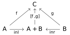
Note that this diagram is like the dual of the diagram seen in the universal property for products — the arrows are reversed. That is because, generally speaking, sums are dual to products. However, because of our additional \bot value, our cpo sums are only weakly universal — the h arrow is not unique.
ExampleWeak universality of cpo sums [dt-003A]
Consider this scenario with the cpos \textbf {2} = \{ \top , \bot \} and \textbf {1} = \{\bot \}:
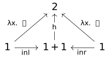
DefinitionWeak universal property for cpo sums [dt-003B]
This property is called weak because it uses only the information ordering rather than equality on the right hand side.
WarningFailure of sum isomorphisms [dt-003C]
The weakness of the universal property for sums means that many common isomorphisms for sums in other contexts do not hold:
- A + (B + C) \not \simeq (A + B) + C
- (A \twoheadrightarrow C) \times (B \twoheadrightarrow C) \not \simeq (A+B) \twoheadrightarrow C
Sums form a bifunctor [dt-0036]
With these, we can define the morphism mapping for the sum bifunctor (+) : \textbf {Cpo} \times \textbf {Cpo} \rightarrow \textbf {Cpo}. Just as with products and functions, we will overload the + notation for morphisms as well as objects in the category \mathbf {Cpo}.
DefinitionSum of functions [dt-0037]
Given functions f : A \twoheadrightarrow C and g : B \twoheadrightarrow D, we have: \begin {array}{l} f+g : (A + B)\twoheadrightarrow (C + D) \\ f+g = [\mathit {inl} \circ f, \mathit {inr} \circ g] \end {array}
Theorem [dt-0038]
+ : \mathbf {Cpo} \times \mathbf {Cpo} \rightarrow \mathbf {Cpo} is a lawful bifunctor, that is:
- (\lambda a. a) \times (\lambda b. b) = (\lambda x.x)
- (f_1 \circ g_1) \times (f_2 \circ g_2) = (f_1 \times f_2) \circ (g_1 \times g_2)
Upshot.
Our category \mathbf {Cpo} has only local sums.
Strict Constructions [dt-003E]
When giving a semantics to a call-by-name (or "lazy") language, the constructions \twoheadrightarrow for functions, \times for products and + for sums are exactly what we want. To properly capture call-by-value (or "strict") languages, however, we also need strict versions of these constructions.
ConstructionThe cpo of strict continuous functions [dt-003F]
The ordering and lubs are, mutatis mutandis, as with the non-strict Construction [dt-002L].
ConstructionSmash products of cpos [dt-003G]
The ordering and lubs are, mutatis mutandis, as with the non-strict Construction [dt-0021]. This operator is called a smash product because the two \bot values from A and B are "smashed" into one \bot value.
ConstructionSmash sums of cpos [dt-003H]
The ordering and lubs are, mutatis mutandis, as with the non-strict Construction [dt-0031]. This operator is called a smash sum because the two \bot values from A and B are "smashed" into one \bot value.
TheoremIsomorphisms with strict constructions [dt-003J]
The strict cpo constructions satisfy all the usual isomorphisms, including:
- (A \mathbin {\circ \hspace{-0.4em}\twoheadrightarrow } B) \times (A \mathbin {\circ \hspace{-0.4em}\twoheadrightarrow } C)\;\; \simeq \;\; A \mathbin {\circ \hspace{-0.4em}\twoheadrightarrow } (B\otimes C)
- (A \otimes B \mathbin {\circ \hspace{-0.4em}\twoheadrightarrow } C) \;\; \simeq \;\; A \mathbin {\circ \hspace{-0.4em}\twoheadrightarrow } (B \mathbin {\circ \hspace{-0.4em}\twoheadrightarrow } C)
- (A \mathbin {\circ \hspace{-0.4em}\twoheadrightarrow } C) \times (B \mathbin {\circ \hspace{-0.4em}\twoheadrightarrow } C)\;\; \simeq \;\; (A\oplus B) \mathbin {\circ \hspace{-0.4em}\twoheadrightarrow } C
DefinitionThe category \mathbf {Cpo_\bot } [dt-003I]
The category \mathbf {Cpo_\bot } is the category where the objects are cpos, the morphisms are strict continuous functions between these cpos, and composition and identity are as in \mathbf {Cpo}.
Upshot.
DefinitionThe lifting operator for cpos [dt-003K]
TheoremIsomorphisms with lifting [dt-003L]
With the lifting operator, we can relate the lazy constructions like product and sum with strict constructions like smash product and sum via isomorphism:
- A\twoheadrightarrow B \simeq A_\bot \mathbin {\circ \hspace{-0.4em}\twoheadrightarrow } B
- A + B \simeq A_\bot \oplus B_\bot
- (A \times B)_\bot \simeq A_\bot \otimes B_\bot
PCF [dt-003T]
For most purposes in semantics, describing semantics in terms of (continuous functions on) cpos is enough. To demonstrate, we will give semantics to PCF: a Turing-complete, higher order functional programming language. We will then extend PCF to include more features, namely pairs (product types) and sum types.
DefinitionThe language PCF [dt-003M]
The language for Programming Computable Functions (PCF) is a variant of typed \lambda -calculus with minimal extensions to be Turing-complete. \begin {array}{lcl} e & \Coloneqq & n \mid x \mid \lambda x : \tau .\ e \mid e_1\ e_2\mid \mathsf {succ} \mid \mathsf {pred} \mid \mathsf {ifz}\ e_1\ \mathsf {then}\ e_2\ \mathsf {else}\ e_3 \mid \mathsf {fix}\ x : \tau .\ e \\ \tau & \Coloneqq & \mathsf {nat} \mid \tau _1 \rightarrow \tau _2 \end {array}
DefinitionTyping rules for PCF [dt-003N]
\dfrac {n \in \mathbb {N}}{\Gamma \vdash n : \mathsf {nat}}\quad \dfrac {x : \tau \in \Gamma }{\Gamma \vdash x : \tau }\quad \dfrac {\Gamma , x : \tau _1 \vdash e : \tau _2 }{ \Gamma \vdash \lambda x : \tau _1.\ e : \tau _1 \rightarrow \tau _2}\quad \dfrac {\Gamma \vdash e_1 : \tau _1 \rightarrow \tau _2 \quad \Gamma \vdash e_2 : \tau _1}{\Gamma \vdash e_1\ e_2 : \tau _2}\\[2em] \dfrac { }{ \Gamma \vdash \mathsf {succ} : \mathsf {nat} \rightarrow \mathsf {nat}}\quad \dfrac { }{ \Gamma \vdash \mathsf {pred} : \mathsf {nat} \rightarrow \mathsf {nat}}\quad \dfrac { \Gamma \vdash e_1 : \mathsf {nat} \quad \Gamma \vdash e_2 : \tau \quad \Gamma \vdash e_3 : \tau }{ \Gamma \vdash \mathsf {ifz}\ e_1\ \mathsf {then}\ e_2\ \mathsf {else}\ e_3 : \tau }\quad \dfrac { \Gamma , x : \tau \vdash e : \tau }{\Gamma \vdash \mathsf {fix}\ x : \tau .\ e : \tau }
Type-dependent denotations [dt-003O]
Because PCF is typed, we shall assign denotations only to well-typed expressions. The range of our denotation function for expressions is determined by the type of its input expression. That is, the denotation of a type \tau is the cpo whose elements will be the denotations of expressions of type \tau . The denotation of the type \mathsf {nat}, then, is merely the flat domain of the natural numbers \mathbb {N}_\bot : \llbracket \mathsf {nat} \rrbracket = \mathbb {N}_\bot And, the denotation of the function type is the domain of continuous functions on cpos: \llbracket \tau _1 \rightarrow \tau _2 \rrbracket = \llbracket \tau _1 \rrbracket \twoheadrightarrow \llbracket \tau _2 \rrbracket A closed term e : \tau with no free variables denotes an element of \llbracket \tau \rrbracket , so we might be tempted to define our denotation function for expressions e : \tau like so: \llbracket e \rrbracket : \llbracket \tau \rrbracket However, if e : \tau involves free variables from our context \Gamma , the valuation of e will depend on the values assigned to all the variables. Thus, the denotation of a typed expression \Gamma \vdash e : \tau is defined instead as a continuous function: \llbracket e \rrbracket _\Gamma : \llbracket \Gamma \rrbracket \twoheadrightarrow \llbracket \tau \rrbracket where the meaning of a context \Gamma = (x_0 : \tau _0, x_1 : \tau _1,\dots , x_n : \tau _n) will be a a big n-tuple of the values assigned to each variable: \llbracket \Gamma \rrbracket = \llbracket \tau _0 \rrbracket \times \llbracket \tau _1 \rrbracket \times \cdots \times \llbracket \tau _n \rrbracket
DefinitionNotation for n-tuples [dt-003Q]
Given an n-tuple, i.e. elements of the n-ary product X_0 \times X_1 \times X_2 \times \dots \times X_n, we typically denote the entire n-tuple as in vector notation: \vec {x} : X_0 \times X_1 \times X_2 \times \dots \times X_n And individual elements of the tuple are accessed with numeric subscripts: x_0 : X_0 \quad x_2 : X_2 \quad \cdots
DefinitionSemantics of PCF [dt-003P]
Types
Expressions
Extending PCF with product types [dt-003R]
We shall extend the syntax of PCF with a new type former, \tau _1 \times \tau _2 and three expression-level constructs for constructing and deconstructing pairs: \begin {array}{lcl} e & \Coloneqq & \cdots \mid (e_1,e_2) \mid \mathsf {fst}\ e \mid \mathsf {snd}\ e \\ \tau & \Coloneqq & \cdots \mid \tau _1 \times \tau _2 \end {array} Adding to our typing rules similarly: \dfrac {\Gamma \vdash e_1 : \tau _1 \quad e_2 : \tau _2}{(e_1,e_2) : \tau _1 \times \tau _2}\\[2em] \dfrac {\Gamma \vdash e : \tau _1 \times \tau _2}{\Gamma \vdash \mathsf {fst}\ e : \tau _1}\quad \dfrac {\Gamma \vdash e : \tau _1 \times \tau _2}{\Gamma \vdash \mathsf {snd}\ e : \tau _2} To extend our semantics, we make the product type \tau _1 \times \tau _2 denote the product cpo \llbracket \tau _1 \rrbracket \times \llbracket \tau _2 \rrbracket , and our expression semantics are expressed straightforwardly using our projection and split operations for products: \begin {array}{lcl} \llbracket (e_1, e_2) \rrbracket _\Gamma &=& \langle \llbracket e_1 \rrbracket _\Gamma , \llbracket e_2 \rrbracket _\Gamma \rangle \\ \llbracket \mathsf {fst}\ e \rrbracket _\Gamma & = & \pi _0 \circ \llbracket e \rrbracket _\Gamma \\ \llbracket \mathsf {snd}\ e \rrbracket _\Gamma & = & \pi _1 \circ \llbracket e \rrbracket _\Gamma \\ \end {array}
Extending PCF with sum types [dt-003S]
We shall extend the syntax of PCF with a new type former, \tau _1 + \tau _2 and three expression-level constructs for constructing and deconstructing sums: \begin {array}{lcl} e & \Coloneqq & \cdots \mid \mathsf {inl}\ e \mid \mathsf {inr}\ e \mid \mathsf {case}\ e_0\ \mathsf {of}\ \mathsf {inl}\ x \rightarrow e_1 ; \mathsf {inr}\ y \rightarrow e_2 \\ \tau & \Coloneqq & \cdots \mid \tau _1 + \tau _2 \end {array} Adding to our typing rules similarly: \dfrac {\Gamma \vdash e : \tau _1}{\Gamma \vdash \mathsf {inl}\ e : \tau _1 + \tau _2}\quad \dfrac {\Gamma \vdash e : \tau _2}{\Gamma \vdash \mathsf {inr}\ e : \tau _1 + \tau _2}\\[2em] \dfrac {\Gamma \vdash e_0 : \tau _1 + \tau _2 \quad \Gamma , x : \tau _1 \vdash e_1 : \tau \quad \Gamma , y : \tau _2 \vdash e_2 : \tau }{ \Gamma \vdash \mathsf {case}\ e_0\ \mathsf {of}\ \mathsf {inl}\ x \rightarrow e_1 ; \mathsf {inr}\ y \rightarrow e_2 : \tau } To extend our semantics, we make the sum type \tau _1 + \tau _2 denote the sum cpo \llbracket \tau _1 \rrbracket + \llbracket \tau _2 \rrbracket , and our expression semantics are expressed using our primitive functions for sums. \begin {array}{lcl} \llbracket \mathsf {inl}\ e \rrbracket _\Gamma & = & \mathit {inl} \circ \llbracket e \rrbracket _\Gamma \\ \llbracket \mathsf {inr}\ e \rrbracket _\Gamma & = & \mathit {inr} \circ \llbracket e \rrbracket _\Gamma \end {array} \begin {array}{l}\llbracket \mathsf {case}\ e_0\ \mathsf {of}\ \mathsf {inl}\ x \rightarrow e_1 ; \mathsf {inr}\ y \rightarrow e_2 \rrbracket _\Gamma (\vec {z}) \\ \quad = [ \boldsymbol {\lambda }v. \llbracket e_1 \rrbracket _{\Gamma ,x:\tau _1}(\vec {z},v), \boldsymbol {\lambda }v. \llbracket e_2 \rrbracket _{\Gamma ,y:\tau _2}(\vec {z},v)] (\llbracket e_0 \rrbracket _\Gamma (\vec {z}))\end {array}