Lecture. Domain theory › Monadic semantics, Scott domains and nondeterminism [dt-005V]
This lecture is based on material from Carl Gunter, Glynn Winskel, Graham Hutton, Kai Engelhardt, Dexter Kozen, Andrew Myers, John Longley, Dana Scott, and Joseph Stoy.
Generalising our semantics [dt-005Z]
We return to the \mathcal {C} language we saw previously:
DefinitionThe \mathcal {C} Language [dt-005R]
Using notation similar to Backus-Naur Form (BNF): \begin {array}{lcl} \mathcal {E} & \Coloneqq & n \mid x \mid \mathcal {E}_1 + \mathcal {E}_2 \mid \mathcal {E}_1 - \mathcal {E}_2\\ \mathcal {B} & \Coloneqq & \mathsf {false} \mid \mathsf {true} \mid \neg \mathcal {B} \mid \mathcal {E}_1 = \mathcal {E}_2\\ \mathcal {C} & \Coloneqq & \mathsf {skip} \mid x := \mathcal {E} \mid \mathcal {C}_1 ; \mathcal {C}_2 \mid \mathsf {if}\ \mathcal {B}\ \mathsf {then}\ \mathcal {C}_1\ \mathsf {else}\ \mathcal {C}_2 \mid \mathsf {while}\ \mathcal {B}\ \mathsf {do}\ \mathcal {C}\ \mathsf {od}\\ x & \in & \mathcal {V}\; \textit {(variables)}\\ n & \in & \mathbb {N} \end {array}
If we wish to add other kinds of effects (beyond mutation of state) to our language, this will necessarily affect the semantic domain. Rather than rewrite the entire semantics for each possible setting, we will generalise the semantics to work over any instance of an algebraic structure, called a monad.
DefinitionMonad [dm-000U]
A monad on the category \textbf {C} consists of an endofunctor \mathcal {M} : \textbf {C} \rightarrow \textbf {C} and two operations (natural transformations) for all \mathbf {C}-objects X: \mu _X : \mathcal {M}(\mathcal {M}(X)) \rightarrow \mathcal {M}(X) and \eta _X : X \rightarrow \mathcal {M}(X), such that the following diagrams commute:
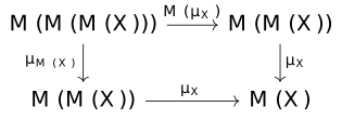
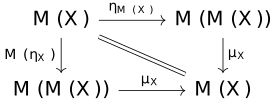
- \mu _X \circ \mathcal {M}(\mu _X) = \mu _X \circ \mu _{\mathcal {M}(X)}
- \mu _X \circ \mathcal {M}(\eta _X) = \mu _X \circ \eta _{\mathcal {M}(X)} = \mathsf {id}_{\mathcal {M}(X)}
ExampleFlat domains as monads [dt-005P]
The flat domain lifting operation (\cdot )_\bot forms a monad, where the endofunctor \mathcal {M}(X) = X_\bot , the operation \mu _X : (X_\bot )_\bot \rightarrow X_\bot collapses the two \bot values, and \eta _X : X \rightarrow X_\bot is simply \eta _X(x) = x.
Sometimes it is more convenient to work with the Kleisli composition operator, rather than the operations \mu and \eta directly.
DefinitionKleisli category [dm-000T]
For a monad (\mathcal {M}, \mu , \eta ) over the category \mathbf {C}, the Kleisli category has the same objects as \mathbf {C}, but the morphisms A \xrightarrow {h} B are those morphisms h of \mathbf {C} that have the form A \xrightarrow {h} \mathcal {M}(B). Composition is defined as follows, for morphisms A \xrightarrow {f} \mathcal {M}(B) and B \xrightarrow {g} \mathcal {M}(C): g \circ _K f = \mu _C \circ \mathcal {M}(g) \circ f Identity morphisms for this category are just \eta .
DefinitionMonadic semantics for \mathcal {C} [dt-005Q]
We define our semantics generically in terms of a monad (\mathcal {M},\mu ,\eta ), using the Kleisli composition operator for \mathcal {M}: \begin {array}{l} \mathsf {ite} : (\Sigma \rightarrow \mathbb {B}) \times (\Sigma \rightarrow \mathcal {M}(\Sigma )) \times (\Sigma \rightarrow \mathcal {M}(\Sigma )) \rightarrow (\Sigma \rightarrow \mathcal {M}(\Sigma ))\\ \mathsf {ite}(b,t,e)(\sigma ) = \begin {cases}t(\sigma ) & \text {if}\ b(\sigma ) = T \\ e(\sigma ) & \text {otherwise} \end {cases} \end {array} \begin {array}{lcl} \llbracket \cdot \rrbracket _\mathcal {C} : \mathcal {C} \rightarrow \Sigma \rightarrow \mathcal {M}(\Sigma )\\[0.4em] \llbracket \mathsf {skip} \rrbracket _\mathcal {C} & = & \eta _\Sigma \\ \llbracket x := e \rrbracket _\mathcal {C} & = & \boldsymbol {\lambda } \sigma .\ \eta _\Sigma (\sigma \left (x \mapsto \llbracket e \rrbracket _\mathcal {E}\right )) \\ \llbracket c_1 ; c_2 \rrbracket _\mathcal {C} & = & \llbracket c_2 \rrbracket _\mathcal {C} \circ _K \llbracket c_1 \rrbracket _\mathcal {C} \\[0.3em] \llbracket \textsf {if}\ b\ \textsf {then}\ c_1\ \textsf {else}\ c_2 \rrbracket _\mathcal {C} & = & \mathsf {ite}(\llbracket b \rrbracket _\mathcal {B},\llbracket c_1 \rrbracket _\mathcal {C},\llbracket c_2 \rrbracket _\mathcal {C})\\ \llbracket \textsf {while}\ b\ \textsf {do}\ c\ \textsf {od} \rrbracket _\mathcal {C} & = & \mathbf {\mathbf {fix}}(\boldsymbol {\lambda } f.\ \mathsf {ite}(\llbracket b \rrbracket _\mathcal {B}, f \circ _K \llbracket c \rrbracket _\mathcal {C}, \eta _\Sigma ) ) \end {array}
ExampleInstantiating \mathcal {C} with the lifting monad [dt-005S]
Instantiating our monadic semantics where the monad \mathcal {M} is flat domain lifting, we recover our original semantics of \mathcal {C}.
ExampleInstantiating \mathcal {C} with exceptions [dt-005T]
Let us instantiate our monadic semantics with the monad \mathcal {M}(X) = X_\bot \oplus \mathbf {1}, where the added value (from \mathbf {1}) is called \mathsf {fail}. The operation \mu _X : (X_\bot \oplus \mathbf {1})_\bot \oplus \mathbf {1} \rightarrow X_\bot \oplus \mathbf {1} collapses the two possible \bot values to \bot and the two possible \mathsf {fail} values to \mathsf {fail}, and the operation \eta _X : X \rightarrow X_\bot \oplus \mathbf {1} is the straightforward injection.
Then we may extend our language with lightweight exception constructs: \mathcal {C} ::= \dots \mid \mathsf {throw} \mid \mathsf {try}\ \mathcal {C}_1\ \mathsf {catch}\ \mathcal {C}_2 and define their semantics, leaving our existing semantics unchanged: \begin {array}{lcl} \llbracket \mathsf {throw} \rrbracket \ \sigma &=& \mathsf {fail} \\ \llbracket \mathsf {try}\ c_1\ \mathsf {catch}\ c_2 \rrbracket \ \sigma &=& \begin {cases} \llbracket c_2 \rrbracket \ \sigma & \text {if}\ \llbracket c_1 \rrbracket \ \sigma = \mathsf {fail} \\ \llbracket c_1 \rrbracket \ \sigma & \text {otherwise}\end {cases} \end {array}
Nondeterminism
Introduction to nondeterminism [dt-005U]
When modelling programming languages we sometimes require a way to be imprecise about some aspects of a program — usually, this takes the form of non-determinism. Non-determinism can be hard for beginners to grasp, but it typically has to be employed when modelling real programs. For example, suppose we had a greeting program that differed depending on the physical location of the computer: \begin {array}{l} \textsf {\textbf {if}}\ \mathit {currentLocation}() = \text {Korea}\ \textsf {\textbf {then}} \\ \quad \textsf {\textbf {say}}\ \text {``안녕하세요''} \\ \textsf {\textbf {else}} \\ \quad \textsf {\textbf {say}}\ \text {``Hello!''}\\ \textsf {\textbf {fi}} \end {array} If we wanted to mathematically model the behaviour of this program, it would be frightfully inconvenient to include the geography of Earth and the computer's physical location in our model. That's where non-determinism comes in. If we abstract away from the geographical details, and instead regard the program as choosing between the two options based on some unspecified criteria, then we can get away with modelling less, at the cost of some detail: \begin {array}{l} \textsf {\textbf {if}}\ \mathit {???}\ \textsf {\textbf {then}} \\ \quad \textsf {\textbf {say}}\ \text {``안녕하세요''} \\ \textsf {\textbf {else}} \\ \quad \textsf {\textbf {say}}\ \text {``Hello!''}\\ \textsf {\textbf {fi}} \end {array} Such underspecified conditionals are usually called non-deterministic choice, where our conditional \textsf {\textbf {if}}\ \mathit {???}\ \textsf {\textbf {then}}\ P\ \textsf {\textbf {else}}\ Q\ \textsf {\textbf {fi}} is written simply as P + Q.
While we tend to view our physical machines as deterministic automata, the state upon which each decision is deterministically made includes a number of external things which are tedious to model mathematically. We can also use non-determinism to ignore details that we don't care about for our particular domain — a common example is memory allocation, where it is very convenient (for some programs) to think of memory as infinite, and allocation as an operation that can potentially fail, without specifying exactly when and how this failure can occur. This is normally modelled as a choice between successful allocation and a failure state.
Instantiating our semantics for nondeterminism [dt-0060]
Our initial semantics for \mathcal {C} (without loops) was functions on states \Sigma \rightarrow \Sigma . When adding loops, we used a cpo \Sigma \twoheadrightarrow \Sigma _\bot for our semantic domain. Since non-deterministic programs can have more than one outcome, a natural choice of semantic domain would be \Sigma \twoheadrightarrow \mathcal {P}(\Sigma _\bot ) \setminus \emptyset , i.e., functions from an initial state to a non-empty set of possible outcomes.
We can provide \eta and \mu operations for our proposed monad for non-determinism \mathcal {M}(X) = \mathcal {P}(X_\bot ) \setminus \emptyset : \begin {array}{l} \eta : X \rightarrow \mathcal {P}(X_\bot ) \setminus \emptyset \\ \eta (x) = \{ x \}\\ \mu : \mathcal {P}{((\mathcal {P}(X_\bot ) \setminus \emptyset )_\bot )}\rightarrow \mathcal {P}(X_\bot ) \setminus \emptyset \\ \mu (S) = (\bigcup _{X \neq \bot \in S} X) \cup (S \cap \{ \bot \}) \end {array} And, with this semantics, we can easily add a denotation for a non-deterministic choice operator, in terms of union: \llbracket c_1 + c_2 \rrbracket _\mathcal {C} = \lambda \sigma . \llbracket c_1 \rrbracket _\mathcal {C} \sigma \cup \llbracket c_2 \rrbracket _\mathcal {C} \sigma Unfortunately this is only the beginning of our troubles. While we have given a valuation function above, its definition uses \textbf {fix}, and therefore our domain \Sigma \rightarrow \mathcal {M}(\Sigma ) must be a cpo, and all our operations continuous. It is not clear how to order elements of \mathcal {P}(X_\bot ) \setminus \emptyset . A natural choice of ordering would be subset inclusion \subseteq . However, as we lack \emptyset , there is no least element for this ordering. Furthermore, simply using \subseteq as our ordering would mean that the deterministic, terminating program that always returns a single state \{ \sigma \} would be considered less informative than the program that may diverge \{ \bot , \sigma \}. This would make most of our operations non-continuous.
Instead, we shall examine three separate orderings on this set, each of which carries a different view of non-determinism. More generally, we wish to come up with a construction analogous to the powerset operator \mathcal {P}, but for our semantic domains — a powerdomain. However, for these orderings to produce valid partial orders, we require a certain theorem that only applies to a certain class of cpos, called "algebraic" cpos. Thus, we will first introduce a richer class of cpos, called Scott domains, and then return to the problem of non-determinism.
Scott domains [dt-005W]
Compactness and Finiteness [dt-0040]
We begin by formalising the notion of an element in a cpo representing a finite amount of information.
DefinitionBoring and interesting sets [dt-003W]
There are two kinds of directed sets:
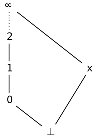
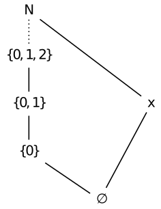
Following the above intuition, we might be tempted to say that the "infinite" elements of a cpo are those which are the lub of an interesting set, but this notion is too weak. Consider this cpo X:
DefinitionCompactness [dt-003U]
Let A be a cpo. Then x \in A is compact (a.k.a. finite) iff for all directed X \subseteq A: x \sqsubseteq \bigsqcup X \implies \exists y \in X.\ x \sqsubseteq y In English: A compact element will approximate some element of a directed set if it approximates the lub. We write \mathsf {K}(A) for the set of compact elements of A, i.e.: \mathsf {K}(A) = \{x \in A \mid x\ \text {is compact} \}
In the example cpo X above, all the elements except \infty and x would be compact. Thus, compactness better captures our notion of an element representing a finite amount of information. This understanding of compact elements is a generalisation of the notion of a finite element from the theory of algebraic lattices.
ExampleCompact elements [dt-003V]
- Every element in a finite cpo is compact. More generally, every element of a cpo of finite height (e.g. \mathbb {Z}_\bot ) is compact. This is because finite directed sets are always boring.
- Take the cpo \mathcal {P}(X) of subsets of X ordered by inclusion \subseteq , as seen in Exercise [dt-001G]. The compact elements of \mathcal {P}(X) are those of finite cardinality.
- Take the cpo \mathbb {N} \nrightarrow \mathbb {N} of partial functions on the natural numbers, ordered by inclusion of graphs. The compact elements of \mathbb {N} \nrightarrow \mathbb {N} are the functions which are defined only for finite domains.
ExampleCompact elements with infinitely many approximations [dt-003X]
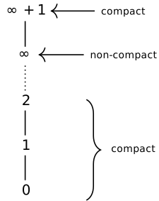
Compact elements may still have an infinite number of approximations. Consider the cpo \mathbb {N} \cup \{ \infty , \infty + 1 \}, where we have tacked on an additional top element \infty + 1 to our normal cpo of natural numbers extended with infinity. Then, while \infty is not compact, \infty + 1 is compact — it is not the lub of an interesting directed set. If \infty + 1 is the lub of a set X then \infty + 1 must be in the set X. Nonetheless, there are an infinite number of approximations to \infty + 1, i.e., elements x such that x \sqsubseteq \infty + 1.
As an aside, requiring that our compact elements have a truly finite number of approximations is the basis for the theory of Berry domains and stable functions.
TheoremSubmonoids as a cpo [dt-003Y]
The submonoids of a monoid (X, \iota , \bullet ) form a cpo under \subseteq , where union gives the lub.
ExerciseBoth infinite and compact [dt-003Z]
Find a set in the cpo of submonoids of (\mathbb {N},0,+) that is both infinite and compact.
Solution.
Take E \triangleq \{ n \in \mathbb {N} \mid n\ \text {is even}\}. Let Y \subseteq \mathcal {P}(\mathbb {N}) be directed and E \subseteq \bigcup Y. Since 2 \in E there must exist y \in Y such that 2 \in Y. Since (y,0,+) is a monoid, every positive multiple of 2 is also in y, thus E \subseteq y and therefore E is compact.
Seeing as compact elements are also sometimes called finite, this is surprising as E is an infinite set. The reason it is nonetheless compact is that E is finitely generated — it is the smallest submonoid of (\mathbb {N},0,+) such that the finite set \{ 2 \} \subseteq E. In fact, the compact submonoids of (\mathbb {N},0,+) are precisely the finitely generated ones.
Algebraicity and ideals [dt-005X]
DefinitionAlgebraicity [dt-0041]
A cpo is algebraic iff every element is the lub of its compact approximations. That is, a cpo D is algebraic iff for all x \in D,
- \mathop {\downarrow }(x) = \{ y \in \mathsf {K}(D) \mid y \sqsubseteq x \} is directed;
- x = \bigsqcup \mathop {\downarrow }(x)
Aside: Plotkin provides an equivalent definition of \omega -algebraic cpos in which directed sets are replaced with \omega -chains throughout. Hutton claims this is less appealing, as the definition speaks of an \omega -chain of compact approximations, rather than the directed set of such.
Example\omega -algebraic cpos [dt-0042]
Many standard examples of cpos are \omega -algebraic cpos: finite cpos, subsets \mathcal {P}(X) of a set X, partial functions \mathbb {N} \nrightarrow \mathbb {N} and submonoids of a monoid. In general, any cpo of subalgebras (e.g. subgroups of a group, subrings of a ring etc.) is \omega -algebraic. This is the origin of the terminology.
CounterexampleNon-algebraic cpo [dt-0043]
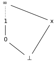
In the cpo on the right (seen also in § [dt-0040]), the element x is not the lub of its compact approximations. The only compact element that approximates x is \bot , and the least upper bound of the set \{\bot \} is just \bot , not x. That is: \mathop {\downarrow }(x) = \{\bot \} but: x \neq \bigsqcup \{\bot \}
TheoremNothing suddenly invented at infinity [dt-0045]
Let D and E be algebraic cpos. Then a function f : D \rightarrow E is continuous iff, for all x \in D: f(x) = \bigsqcup \ \{ f(a) \mid a \in \mathop {\downarrow }(x) \} In other words, in an algebraic cpo, continuous functions are completely defined by their behaviour for compact arguments.
This makes precise our earlier slogan in Definition [dt-001J], that continuous functions don't suddenly behave differently for infinite (i.e. non-compact) elements.
Proof.
Exercise [dt-0044]
Let f : D \twoheadrightarrow E be a continuous function between algebraic cpos. Define: G_f = \{ (a,b) \in \mathsf {K}(D) \times \mathsf {K}(E) \mid b \sqsubseteq f(a) \} Then for all x \in D, prove that: f(x) = \bigsqcup \ \{ b \mid (a,b) \in G_f \land a \sqsubseteq x \}
Solution.
This is powerful. For example, the continuous function f : \mathcal {P}(\mathbb {N}) \twoheadrightarrow \mathcal {P}(\mathbb {N}) on an uncountable cpo \mathcal {P}(\mathbb {N}) is completely determined by the countable relation G_f.
DefinitionDown-closure [dt-0047]
Given a poset Y, a set X \subseteq Y is down-closed iff, for all x \in X, any y \sqsubseteq x is in X.
DefinitionIdeal [dt-0048]
A set is ideal iff it is both down-closed and directed.
DefinitionIdeal completion [dt-0046]
The ideal completion of a set A, written sometimes as \mathsf {Id}(A), is the set of all ideal subsets of A, i.e.: \mathsf {Id}(A) = \{ X \subseteq A \mid X\ \text {is ideal}\}
TheoremRepresentation theorem for algebraic cpos [dt-0049]
Every algebraic cpo D is isomorphic to the ideal completion of its compact elements, ordered by subset inclusion. That is, \mathsf {Id}(K(D)) is an algebraic cpo such that D \simeq \mathsf {Id}(K(D)) .
Getting closure [dt-005Y]
DefinitionBasis [dt-004A]
TheoremCompact basis for algebraic cpos [dt-004B]
If X is a basis for A, then A is algebraic and \mathsf {K}(A) = X.
Proof.
If a \in \mathsf {K}(A), then \bigsqcup M = a where M = \{ x \in X \mid x \sqsubseteq a \}, as X is a basis. Since a is compact, a \sqsubseteq b for some b \in M. But since a is the lub of M, b \sqsubseteq a as well. By antisymmetry a = b, hence a \in X. Thus \mathsf {K}(A) \subseteq X, so \mathsf {K}(A) = X and A is algebraic.
TheoremClosure of algebraic cpos under product [dt-004C]
If D and E are algebraic cpos, then so is their product construction D \times E.
Proof.
In the following proof, we show that \mathsf {K}(D) \times \mathsf {K}(E) is a basis for the product D \times E and thereby show via Theorem [dt-004B] that D \times E is algebraic if D and E are.
- \mathsf {K}(D) \times \mathsf {K}(E) \subseteq \mathsf {K}(D \times E): Let (x,y) \in \mathsf {K}(D) \times \mathsf {K}(E). To show that (x,y) is compact, let us assume that (x,y) \in \bigsqcup X where X \subseteq D \times E is directed. We must show that there exists some element e of X such that our (x,y) \sqsubseteq e. As (x,y) \in \bigsqcup X, by the definition of lub on products we can conclude that:
\begin {array}{lcl}
x & \sqsubseteq & \bigsqcup \pi _0[ X] \\
y & \sqsubseteq & \bigsqcup \pi _1[X]
\end {array}
Here we use the notation f[X] to indicate the image of a function on a set, i.e. \{ f(v) \mid v \in X \}.
Since x and y are both compact, there must exist x' \in \pi _0[ X] and y' \in \pi _1[ X] such that x \sqsubseteq x' and y \sqsubseteq y'. While it does not follow that (x', y') \in X, we know that there must exist a pair (a,b) \in X such that x' \sqsubseteq a and y' \sqsubseteq b as X is directed. Hence (a,b) can be our element e \in X that is approximated by (x,y), i.e. (x,y) \sqsubseteq (a,b). - \mathop {\downarrow }(x,y) is directed for all (x,y) \in D \times E: \begin {array}{lcl} \mathop {\downarrow }(x,y) &= & \{ (a,b) \in \mathsf {K}(D) \times \mathsf {K}(E) \mid (a,b) \sqsubseteq (x,y) \} \\ & = & \{ a \in \mathsf {K}(D) \mid a \sqsubseteq x \} \times \{ b \in \mathsf {K}(E) \mid b \sqsubseteq y \}\\ & = & \mathop {\downarrow }(x) \times \mathop {\downarrow }(y) \end {array} Because D and E are algebraic, \mathop {\downarrow }(x) and \mathop {\downarrow }(y) are directed. As directedness is closed under product, \mathop {\downarrow }(x,y) is directed too.
- (x,y) = \bigsqcup \mathop {\downarrow }(x,y) Starting from the right hand side: \begin {array}{lclr} \bigsqcup \mathop {\downarrow }(x,y) & = & \bigsqcup (\mathop {\downarrow }(x) \times \mathop {\downarrow }(y)) & \text {(part 2)}\\ & = & (\bigsqcup (\mathop {\downarrow }(x), \bigsqcup \mathop {\downarrow }(y))) & \text {(lub on products)}\\ & = & (x,y) & \text {($D$, $E$ are {algebraic})} \end {array}
Problem.
AsideScott's original solution: using complete lattices [dt-004D]
The lack of closure of algebraicity under the (continuous) function arrow, strict or non-strict, is not satisfying as it means that our semantic domains are not guaranteed to be algebraic even if they are composed from algebraic cpos. Instead, we must replace algebraic cpos with something stronger still.
Scott's original solution to this lack of closure was to use a complete lattice instead of cpos, i.e. requiring lubs for all subsets, not just directed ones. This solves the problem with \twoheadrightarrow but introduces new problems:
- Complete lattices need a top element \top , but adding a fictitious top (representing inconsistent information) to cpos like \mathbb {B}_\bot is strange.
- Extending the functions that capture our primitive semantic operations to complete lattices can spoil nice algebraic properties. Consider these two possible implementations of \mathsf {ite}, the function for the semantics of an \mathsf {if} expression: \mathsf {ite}(\top ,x,y) = x \sqcup y\quad \quad \quad \quad \quad \mathsf {ite}(\top ,x,y) = \top Either of these solutions results in the failure of useful and expected laws for \mathsf {if} expressions. For example, the left definition above results in the failure of the common equation to eliminate unreachable cases: \mathsf {ite}(b, \mathsf {ite}(b,x,y),z) = \mathsf {ite}(b,x,z) And the second definition above results in the failure of this equation that removes redundant checks: \mathsf {ite}(b,x,x) = x
- The powerdomain construction does not generalise to complete lattices, so semantics for non-deterministic programs are difficult in this setting.
DefinitionConsistent completeness [dt-004E]
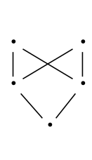
A poset A is consistent complete (or bounded complete) iff \bigsqcup X exists for all consistent X \subseteq A. That is, any set with an upper bound (a consistent set) has a least upper bound.
ExampleConsistent completeness vs directed completeness [dt-004F]

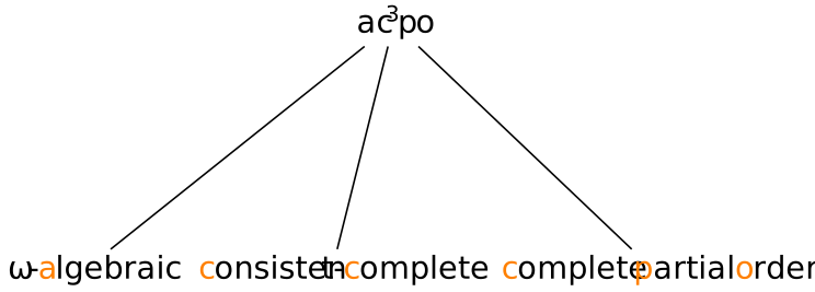
DefinitionScott domain [dt-004G]
A cpo D is a Scott domain iff:
- D is \omega -algebraic,
- D is consistent complete,
Remark [dt-004H]
The second requirement in Definition [dt-004G] can, in light of the first, be expressed equivalently as: x \sqcup y exists for all consistent x,y \in D. This is useful when needing to show that a given cpo is a Scott domain.
TheoremClosure of Scott domains [dt-004I]
Scott domains are closed under all our cpo constructions, including sums +, products \times , continuous functions \twoheadrightarrow , smash sums \oplus , smash products \otimes and strict functions \mathbin {\circ \hspace{-0.4em}\twoheadrightarrow }.
Thesis.
Our semantic domains are Scott domains.
The Hoare powerdomain [dt-0061]
We write \mathcal {P}_f^\ast (S) to denote finite non-empty subsets of S. Let X, Y \in \mathcal {P}_f^\ast (\mathsf {K}(A)) be finite, non-empty sets of compact elements of a Scott domain A. The Hoare powerdomain construction is based on the following ordering: X \preceq _H Y\quad \text {iff}\quad (\forall x \in X.\ \exists y \in Y.\ x \sqsubseteq _A y) The intuition behind this is that "Anything X can do, Y can do better". This ordering has some desirable properties: The least element is \{\bot \}, as we might expect. It also satisfies the equation X \preceq _H X \cup Y, which intuitively means that a non-deterministic choice is considered to have more information than any of its components. When specialised to the case where A is a flat domain like \Sigma _\bot , it simplifies to: X \preceq _H Y\quad \text {iff}\quad X \setminus \{\bot \} \subseteq Y This is, however, not a proper order, but a preorder, as it fails antisymmetry. Even in the flat domain case, \{ x, \bot \} \preceq _H \{x \} and \{ x \} \preceq _H \{x, \bot \} but they are not equal. However, any preorder does induce an equivalence relation, where X \approx _H Y iff X \preceq _H Y and Y \preceq _H X. Furthermore, if we take the ideal completion of \mathcal {P}_f^\ast (K(A)) with respect to the preorder \preceq _H (i.e., the set of all \preceq _H-downwards-closed directed subsets of \mathcal {P}_f^\ast (\mathsf {K}(A))), we can order them by inclusion to obtain an algebraic domain with compact elements which correspond to equivalence classes of elements under \approx _H. We have a lub operation for these ideals: A \sqcup _H B = \{ X \cup Y \mid X \in A \land Y \in B \}
ExampleHoare powerdomain of \mathbb {N}_\bot [dt-0062]
Let us find the Hoare powerdomain of \mathbb {N}_\bot . Note that \mathbb {N}_\bot is a flat domain so all elements are compact, i.e. \mathsf {K}(\mathbb {N}_\bot ) = \mathbb {N}_\bot . Let us find examine the \preceq _H-ideal subsets of \mathcal {P}_f^\ast (\mathbb {N}_\bot ). If v and u both contain \bot , then v \preceq _H u iff v \subseteq u. As ideal subsets are downwards closed, we can identify an ideal I \in \mathsf {Id}({\mathcal {P}_f^\ast (\mathbb {N}_\bot )}) with its union \bigcup I. The ideals of \mathcal {P}^\ast _f(\mathbb {N}_\bot ) are then isomorphic to domain \mathcal {P}(\mathbb {N}) of all subsets of \mathbb {N} under subset inclusion.
RemarkAngelic nondeterminism [dt-0063]
Consider the following three programs:
- x := 1
- \textsf {while}\ \textsf {true}\ \textsf {do}\ \textsf {skip}
- \textsf {while}\ \textsf {true}\ \textsf {do}\ \textsf {skip}\ \textsf {od} + x := 1
The Smyth powerdomain [dt-0064]
As before, let X, Y \in \mathcal {P}_f^\ast (\mathsf {K}(A)) be finite, non-empty sets of compact elements of a Scott domain A. The Smyth powerdomain construction is based on the following preorder: X \preceq _S Y\quad \text {iff}\quad (\forall y \in Y.\ \exists x \in X.\ x \sqsubseteq _A y) The intuition here is "Everything Y can do, X can do worse". It satisfies the equation X \cup Y \preceq _S X, which intuitively means that a non-deterministic choice is considered to have less information than any of its components. When applied to a flat domain, it simplifies to: X \preceq _S Y\quad \text {iff}\quad \bot \in X \lor Y \subseteq X As with the Hoare powerdomain, this fails to be a partial order, but we can use the same ideal completion trick to induce an algebraic domain where compact elements correspond to equivalence classes of elements under \approx _S (where X \approx _S Y is, as with \approx _H, just defined as X \preceq _S Y \land Y \preceq _S X).
ExampleSmyth powerdomain of \mathbb {N}_\bot [dt-0065]
Firstly note that, as ideals are downwards-closed, any \preceq _S-ideal subsets of \mathcal {P}^\ast _f(\mathbb {N}_\bot ) will contain all finite subsets of \mathbb {N}_\bot that contain \bot . Let us call those sets trivial. So, a set in \mathcal {P}^\ast _f(\mathbb {N}_\bot ) is non-trivial if it does not contain \bot and an ideal subset of \mathcal {P}^\ast _f(\mathbb {N}_\bot ) is non-trivial if it contains a non-trivial set. Observe that for non-trivial sets X and Y, X \preceq _S Y iff X \supseteq Y. Thus, we can identify an ideal I \in \mathsf {Id}({\mathcal {P}_f^\ast (\mathbb {N}_\bot )}) with the down-closure of the intersection of its non-trivial elements. The smaller this set is, the larger the ideal I. Hence, and confusingly, the non-trivial ideals in the powerdomain (ordered by subset inclusion) correspond to finite subsets of \mathbb {N} ordered by superset inclusion. As all trivial sets are identified, we just need to throw in the unique trivial ideal, and we can see that the Smyth powerdomain of \mathbb {N} is isomorphic to the domain of sets \{ \mathbb {N} \} \cup \mathcal {P}_f^\ast (\mathbb {N}) ordered by subset inclusion.
RemarkDemonic nondeterminism [dt-0066]
Note that all sets that contain \bot are considered equivalent by the Smyth construction \approx _S. Thus, this models demonic non-determinism: Of the three programs in Remark [dt-0063], the Smyth semantics considers 2 and 3 to be the same. Thus, the possibility of divergence \bot is no different from inevitable divergence.
The Plotkin powerdomain [dt-0067]
As before, let X, Y \in \mathcal {P}_f^\ast (\mathsf {K}(A)) be finite, non-empty sets of compact elements of a Scott domain A. The Plotkin powerdomain construction is based on the following preorder, simply combining the orderings from the Hoare and Smyth constructions: X \preceq _P Y\quad \text {iff}\quad X \preceq _H Y \land X \preceq _S Y This ordering is also called the Egli-Milner ordering. On a flat domain, it simplifies to: A\sqsubseteq B\quad \text {iff}\quad A = B \lor (\bot \in A \land (A \setminus \{\bot \})\subseteq B) Note that this is antisymmetric in the case of a flat domain, and the lub of a chain of sets can be found by taking the union of all elements of the chain if all elements contain \bot If not, then the element without \bot will be the least upper bound.
The failures of antisymmetry can only be observed in domains of height higher than one. Consider a set \{x,y\} containing two elements. According to the induced equivalence from this preorder \approx _P, this set would be considered equal to the set that contains those two elements plus any elements that lie between them on the information ordering: \{x,y\} \approx _P \{ z \mid x \sqsubseteq z \sqsubseteq y \} The Plotkin powerdomain is sometimes called the convex powerdomain, due to the similarity of this to the geometric definition of convexity. Thus, we use the ideal completion trick (as with the Hoare and Smyth constructions) here to arrive at a definition of powerdomain that distinguishes between all three programs outlined in Remark [dt-0063].
Aside.
There is a beautiful algebraic characterisation of Plotkin powerdomains in Matthew Hennessy Gordon Plotkin's paper, Full abstraction for a simple parallel programming language.